Download

1 / 23
240 likes | 350 Views
Learn about Generalized Additive Models, comparison with GLMs, efficient algorithms like splines, ozone pollution example, flexible modeling with optimal solutions, ANOVA analysis, and possible refinements for better results.

E N D
Advanced Research Skills Lecture 8 Generalized Additive Models Olivier MISSA, om502@york.ac.uk
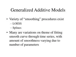
Outline • Introduce you to Generalized Additive Models.
GAMs vs. GLMs • GLMs • GAMs Smooth function of x1
"Smooth" functions • A number of algorithms are available to fit them, • all known generically as "splines" • The most frequently used are: • Thin Plate Regression Splines (default) & • Cubic Regression Splines
degree 10 degree 5 More efficient than Polynomials Thin Plate Regression Splines Est. degr. freedom : 8.69 R2 (adj) : 0.783 Dev. Expl. :79.8% Polynomials degr. freedom : 10 R2 (adj) : 0.762 Dev. Expl. : 78%
More efficient than Polynomials No need to specify the degrees of freedom (Wiggliness) of the smooth function. The algorithm finds the optimal solution for us, and avoids overfitting by cross-validation ('leave-one-out' trick).
Example: ozone pollution • Revisiting the ozone dataset (Lecture 4 Linear Models III) > ozone.pollution <- read.table("ozone.data.txt", header=T) ## in datasets folder > names(ozone.pollution) [1] "rad" "temp" "wind" "ozone" > attach(ozone.pollution) > modgam <- gam(ozone ~ s(rad) + s(temp) + s(wind) ) > plot(ozone ~ modgam$$fitted, pch=16) > abline(0,1, col="red")
Generalised Cross-Validation Ozone Example > summary(modgam) Family: gaussian Link function: identity ... Parametric coefficients: Estimate Std. Error t value Pr(>|t|) (Intercept) 42.10 1.66 25.36 <2e-16 *** --- ... Approximate significance of smooth terms: edf Ref.df F p-value s(rad) 2.763 3.263 4.106 0.00699 ** s(temp) 3.841 4.341 12.785 7.31e-09 *** s(wind) 2.918 3.418 14.687 1.21e-08 *** R-sq.(adj) = 0.724 Deviance explained = 74.8% GCV score = 338 Scale est. = 305.96 n = 111
temp rad wind Ozone Example > plot(modgam, residuals=T, pch=16) > modgam2 <- update(modgam, ~. - s(rad) ) > modgam3 <- update(modgam, ~. - s(temp) ) > modgam4 <- update(modgam, ~. - s(wind) )
Ozone Example > anova(modgam, modgam2, test="F") Model 1: ozone ~ s(rad) + s(temp) + s(wind) Model 2: ozone ~ s(temp) + s(wind) Resid. Df Resid. Dev Df Deviance F Pr(>F) 1 100.4779 30742 2 102.8450 34885 -2.3672 -4142 5.7192 0.002696 ** > anova(modgam, modgam3, test="F") Model 1: ozone ~ s(rad) + s(temp) + s(wind) Model 2: ozone ~ s(rad) + s(wind) Resid. Df Resid. Dev Df Deviance F Pr(>F) 1 100.4779 30742 2 104.7320 47967 -4.2541 -17224 13.233 5.141e-09 *** > anova(modgam, modgam4, test="F") Model 1: ozone ~ s(rad) + s(temp) + s(wind) Model 2: ozone ~ s(rad) + s(temp) Resid. Df Resid. Dev Df Deviance F Pr(>F) 1 100.4779 30742 2 103.5741 46942 -3.0962 -16199 17.1 3.218e-09 ***
Ozone Example > modgam5 <- gam(ozone ~ rad + s(temp) + s(wind) ) > summary(modgam5) Family: gaussian Link function: identity ... Parametric coefficients: Estimate Std. Error t value Pr(>|t|) (Intercept) 30.21525 4.03762 7.483 2.57e-11 *** rad 0.06431 0.01985 3.239 0.00162 ** --- Approximate significance of smooth terms: edf Ref.df F p-value s(temp) 3.448 3.948 14.77 1.73e-09 *** s(wind) 2.912 3.412 15.35 5.56e-09 *** --- R-sq.(adj) = 0.715 Deviance explained = 73.4% GCV score = 341.18 Scale est. = 315.48 n = 111 linear term
Ozone Example > anova(modgam, modgam5, test="F") Analysis of Deviance Table Model 1: ozone ~ s(rad) + s(temp) + s(wind) Model 2: ozone ~ rad + s(temp) + s(wind) Resid. Df Resid. Dev Df Deviance F Pr(>F) 1 100.4779 30742 2 102.6408 32381 -2.1630 -1639 2.4766 0.0848 . --- > shapiro.test(residuals(modgam5, type="deviance")) Shapiro-Wilk normality test data: residuals(modgam5, type = "deviance") W = 0.9123, p-value = 1.999e-06 > resid <- residuals(modgam5, type="deviance")
Ozone Example > qqnorm(resid, pch=16) > qqline(resid, lwd=2, col="red") > plot(resid ~ fitted(modgam5), pch=16) > abline(h=0, col="gray85", lty=2)
Ozone Example > plot(sqrt(abs(resid)) ~ fitted(modgam5), pch=16) > lines(lowess(sqrt(abs(resid)) ~ fitted(modgam5)), lwd=2, col="red") > plot(cooks.distance(modgam5), type="h")
Possible Refinements Specify a different family than Gaussian > modgam <- gam(resp ~ pred1 + s(pred2) + s(pred3), family=poisson(link="log") ) cubic regression spline Specify a different spline basis than Thin Plate > modgam <- gam(resp ~ pred1 + s(pred2, bs="cr") + s(pred3) ) Specify a maximum number of degrees of freedom for the spline > modgam <- gam(resp ~ pred1 + s(pred2, k=5) + s(pred3) )
1st Example > plot( c(0,1) ~ c(1,32), type="n", log="x", xlab="dose", ylab="Probability") > text(dose, numdead/20, labels=as.character(sex) ) > ld <- seq(0,32,0.5) > lines (ld, predict(modb3, data.frame(ldose=log2(ld), sex=factor(rep("M", length(ld)), levels=levels(sex))), type="response") ) > lines (ld, predict(modb3, data.frame(ldose=log2(ld), sex=factor(rep("F", length(ld)), levels=levels(sex))), type="response"), lty=2, col="red" )
1st Example > modbp <- glm(SF ~ sex*ldose, family=binomial(link="probit")) > AIC(modbp) [1] 41.87836 > modbc <- glm(SF ~ sex*ldose, family=binomial(link="cloglog")) > AIC(modbc) [1] 43.8663 > AIC(modb3) [1] 42.86747
1st Example > summary(modb3) Coefficients: Estimate Std. Error z value Pr(>|z|) (Intercept) -3.4732 0.4685 -7.413 1.23e-13 *** sexM 1.1007 0.3558 3.093 0.00198 ** ldose 1.0642 0.1311 8.119 4.70e-16 *** --- > exp(modb3$coeff) ## careful it may be misleading (Intercept) sexM ldose 0.031019 3.006400 2.898560 ## odds ration: p / (1-p) > exp(modb3$coeff[1]+modb3$coeff[2]) ## odds for males (Intercept) 0.09325553 logit scale Every doubling of the dose will lead to an increase in the odds of dying over surviving by a factor of 2.899
2nd Example • Erythrocyte Sedimentation Rate in a group of patients. • Two groups : <20 (healthy) or >20 (ill) mm/hour • Q: Is it related to globulin & fibrinogen level in the blood ? > data("plasma", package="HSAUR") > str(plasma) 'data.frame': 32 obs. of 3 variables: $ fibrinogen: num 2.52 2.56 2.19 2.18 3.41 2.46 3.22 2.21 ... $ globulin : int 38 31 33 31 37 36 38 37 39 41 ... $ ESR : Factor w/ 2 levels "ESR < 20","ESR > 20": 1 1 ... > summary(plasma) fibrinogen globulin ESR Min. :2.090 Min. :28.00 ESR < 20:26 1st Qu.:2.290 1st Qu.:31.75 ESR > 20: 6 Median :2.600 Median :36.00 Mean :2.789 Mean :35.66 3rd Qu.:3.167 3rd Qu.:38.00 Max. :5.060 Max. :46.00
2nd Example > stripchart(globulin ~ ESR, vertical=T, data=plasma, xlab="Erythrocyte Sedimentation Rate (mm/hr)", ylab="Globulin blood level", method="jitter" ) > stripchart(fibrinogen ~ ESR, vertical=T, data=plasma, xlab="Erythrocyte Sedimentation Rate (mm/hr)", ylab="Fibrinogen blood level", method="jitter" )
2nd Example factor > mod1 <- glm(ESR~fibrinogen, data=plasma, family=binomial) > summary(mod1) Coefficients: Estimate Std. Error z value Pr(>|z|) (Intercept) -6.8451 2.7703 -2.471 0.0135 * fibrinogen 1.8271 0.9009 2.028 0.0425 * --- (Dispersion parameter for binomial family taken to be 1) Null deviance: 30.885 on 31 degrees of freedom Residual deviance: 24.840 on 30 degrees of freedom AIC: 28.840 > mod2 <- glm(ESR~fibrinogen+globulin, data=plasma, family=binomial) > AIC(mod2) [1] 28.97111
2nd Example > anova(mod1, mod2, test="Chisq") Analysis of Deviance Table Model 1: ESR ~ fibrinogen Model 2: ESR ~ fibrinogen + globulin Resid. Df Resid. Dev Df Deviance P(>|Chi|) 1 30 24.8404 2 29 22.9711 1 1.8692 0.1716 > summary(mod2) Coefficients: Estimate Std. Error z value Pr(>|z|) (Intercept) -12.7921 5.7963 -2.207 0.0273 * fibrinogen 1.9104 0.9710 1.967 0.0491 * globulin 0.1558 0.1195 1.303 0.1925 --- (Dispersion parameter for binomial family taken to be 1) Null deviance: 30.885 on 31 degrees of freedom Residual deviance: 22.971 on 29 degrees of freedom AIC: 28.971 The difference in terms of Deviance between these models is not significant, which leads us to select the least complex model
2nd Example > shapiro.test(residuals(mod1, type="deviance")) Shapiro-Wilk normality test data: residuals(mod1, type = "deviance") W = 0.6863, p-value = 5.465e-07 > par(mfrow=c(2,2)) > plot(mod1)