Download
1 / 39
390 likes | 396 Views
This study examines the importance of accurate cloud observations in climate modeling and highlights the challenges in obtaining consistent long-term cloud data. It compares satellite observations with other datasets and explores the effects of factors like orbit drift, CO2 increase, and sensor changes.

E N D
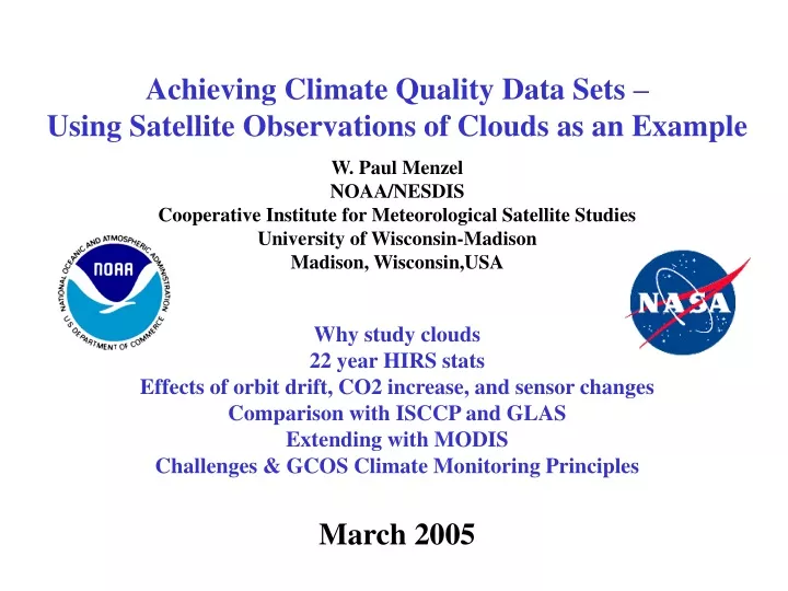
Achieving Climate Quality Data Sets – Using Satellite Observations of Clouds as an Example W. Paul Menzel NOAA/NESDIS Cooperative Institute for Meteorological Satellite Studies University of Wisconsin-Madison Madison, Wisconsin,USA Why study clouds 22 year HIRS stats Effects of orbit drift, CO2 increase, and sensor changes Comparison with ISCCP and GLAS Extending with MODIS Challenges & GCOS Climate Monitoring Principles March 2005
Rationale for Cloud Investigations clouds are a strong modulator of shortwave and longwave; their effect on global radiative processes is large (1% change in global cloud cover equivalent to about 4% change in CO2 concentration) accurate determination of global cloud cover has been elusive (semi transparent clouds often underestimated by 10%) global climate change models need accurate estimation of cloud cover, height, emissivity, thermodynamic state, particle size (high/low clouds give positive/negative feedback to greenhouse effect, and higher albedo from anthropogenic aerosols may be negative feedback) there is a need for consistent long term observation records to enable better characterization of weather and climate variability (ISSCP is a good start)
Why are clouds so tough? • Aerosols <0.1 micron, cloud systems >1000 km • Cloud particles grow in seconds: climate is centuries • Cloud growth can be explosive: 1 thunderstorm packs the energy of an H-bomb. • Cloud properties can vary a factor of 1000 in hours. • Few percent cloud changes drive climate sensitivity • Best current climate models are 250 km scale • Cloud updrafts are a 100 m to a few km.
Inferring Decadal HIRS Cloud Trends requires corrections for (1) anomalous satellite data or gaps (2) orbit drift (3) CO2 increase constant CO2 concentration was assumed in analysis
Satellite by satellite analysis Gap in 8am/pm orbit coverage between NOAA-8 and -10 HIRS cloud trends show unexplained dip with NOAA-7 in 2 am/pm orbit. Used only 2 am/pm orbit data after 1985 in cloud trend analysis for continuity of data and satellite to satellite consistency
Measurements from 9 sensors used in 22 year study of clouds morning (8 am LST)afternoon (2 pm LST) NOAA 6 HIRS/2 NOAA 5 HIRS NOAA 8 HIRS/2 NOAA 7 HIRS/2 NOAA 10 HIRS/2 NOAA 9 HIRS/2 NOAA 12 HIRS/2 NOAA 11 HIRS/2I * NOAA 14 HIRS/2I * HIRS/2I ch 10 at 12.5 um instead of prior HIRS/2 8.6 um. Asterisk indicates orbit drift from 14 UTC to 18 UTC over 5 years of operation Some sensors experienced significant orbit drift
all 2 am/pm satellites adjusted linearly to represent data for ascending node at 1400 hrs local time
Atmospheric CO2 has not been constant (From Engelen et al., Geophys Res Lett, 2001)
SARTA calculations: BT with 360 ppmv minus BT with 340,345,…380 ppmv
HIRS cloud trends have been calculated with CO2 concentration assumed constant at 380 ppm. • Lower CO2 concentrations increase the atmospheric transmission, so radiation is detected from lower altitudes in the atmosphere. • dry(335,p,ch) = dry(380,p,ch)**{335/380) • (p,ch) = dry(p,ch)*H2O(p,ch)*O3(p,ch). • For January and June 2001 the clouds detected by NOAA 14 in the more transparent atmosphere (CO2 at 335 ppm) are found to be lower by 15-50 hPa • More transparent atmosphere (CO2 at 335 ppm) results in HIRS reporting • 2% less high clouds than in the more opaque atmosphere (CO2 at 380 ppm); this implies that the frequency of high cloud detection in the early 1980s should be adjusted down. • Cloud time series was adjusted to represent a linear increase of CO2 from 335 ppm in 1979 to 375 ppm in 2001
The monthly average frequency of clouds and high clouds (above 6 km) from 70 south to 70 north latitude from 1979 to 2002; Wylie et al 2005.
Frequency of all clouds found in HIRS data since 1979 Change in cloud frequency from the 1980s to the 1990s Change in high cloud (above 6 km) frequency during northern hemisphere winters Wylie et al 2005
High cloud (above 6 km) frequency during El Nino years (top) compared with all other years (bottom) during northern hemisphere winters (December, January, and February) from 1980s to 1990s.
Comparing with ISCCP and GLAS (1) using GLAS as a sanity check (2) understanding ISCCP and algorithm differences
How Cloudy is the Earth? CLAVR 60 GLAS 22 Feb – 28 Mar 2003, HIRS 1979 – 2001, ISCCP 1983 – 2001, SAGE 1985-89, Surface Reports 1980-89, CLAVR 1982 - 2004 ISCCP reports 7-15% less cloud than HIRS because it misses thin cirrus. HIRS and GLAS report nearly the same high cloud frequencies. HIRS reports more clouds over land than GLAS probably because GLAS sees holes in low cumulus below the resolution of HIRS.
All Cloud Observations from GLAS vs HIRS GLAS HIRS
HIRS minus GLAS All Cloud Difference HIRS Frequency of All Clouds during the period of GLAS GLAS finds more tropical clouds over oceans where HIRS reports <40%. GLAS finds less clouds in polar regions and western tropical Pacific.
HIRS minus GLAS High Cloud Difference HIRS Frequency of High Cloud HIRS – GLAS Difference GLAS > HIRS HIRS > GLAS HIRS reports more high clouds in parts of tropics and southern hemisphere, but areas of differences are scattered and not meteorologically organized.
Wylie et al Differences between UW HIRS analysis and the ISCCP are primarily (a) ISCCP uses visible reflectance measurements with the infrared window thermal radiance measurements, which limits transmissive cirrus detection to only day light data; (b) UW HIRS analysis uses only longwave infrared data from 11 to 15 µm which is more sensitive to transmissive cirrus clouds, but is relatively insensitive to low level marine stratus clouds Campbell and VonderHaar ISCCP may be showing fewer clouds as satellite coverage (and hence more nadir viewing coverage) increases in later years.
Extending HIRS Cloud Trends with MODIS requires corrections for (1) improved spatial resolution (2) spectral changes
Summary of AIRS minus MODIS mean Tb differences, 6 Sept 2002 Red=without accounting for ce Blue=accounting for ce with mean correction from standard atmospheres mm Band Band Diff CE Diff Std N 21 0.10 -0.01 0.09 0.23 187487 22 -0.05 -0.00 -0.05 0.10 210762 23 -0.05 0.19 0.14 0.16 244064 24 -0.23 0.00 -0.22 0.24 559547 25 -0.22 0.25 0.03 0.13 453068 27 1.62 -0.57 1.05 0.30 1044122 28 -0.19 0.67 0.48 0.25 1149593 30 0.51 -0.93 -0.41 0.26 172064 31 0.16 -0.13 0.03 0.12 322522 32 0.10 0.00 0.10 0.16 330994 33 -0.21 0.28 0.07 0.21 716940 34 -0.23 -0.11 -0.34 0.15 1089663 35 -0.78 0.21 -0.57 0.28 1318406 36 -0.99 0.12 -0.88 0.43 1980369
Summary of AIRS minus MODIS mean Tb differences, 18 Feb 2004 Red=without accounting for ce Blue=accounting for ce with mean correction from standard atmospheres mm Band Band Diff CE Diff Std N 21 -0.32 -0.01 -0.33 0.18 80388 22 -0.14 -0.00 -0.14 0.25 246112 23 -0.15 0.19 0.04 0.20 277755 24 -0.22 -0.08 -0.30 0.25 511821 25 -0.41 0.38 -0.03 0.18 573261 27 1.24 -0.57 0.67 0.39 1098476 28 -0.29 0.67 0.38 0.21 1250087 30 0.21 -0.91 -0.70 0.23 358698 31 0.19 -0.13 0.06 0.09 393559 32 0.13 -0.01 0.12 0.13 401780 33 -0.15 0.21 0.06 0.16 817442 34 0.01 -0.49 -0.48 0.12 1228199 35 -0.72 0.17 -0.55 0.31 1480551 36 -0.92 0.12 -0.81 0.51 2151789
band 36: +1.0 cm-1 band 35: +0.8 cm-1 band 34: +0.8 cm-1 band 33: -0.15 cm-1 06 Sep 2002: 18 Feb 2004:
Atmospheric transmittance in CO2 sensitive region of spectrum Studying spectral sensitivity with AIRS Data AIRS BT[747.8] – BT[747.4] Spectral change of 0.4 cm-1 causes BT changes > 8 C
Current CTP (HI clouds) White: 95 ~ 125 Red: 125 ~ 160 Orange:160~190 Yellow: 190~225 Aqua: 225 ~ 260 Cyan: 260~300 Sky: 300~ 330 Blue: 330~360 Navy: 360~ 390
CTP with SRF Adjustment (band 34,35,36) (HI clouds) White: 95 ~ 125 Red: 125 ~ 160 Orange:160~190 Yellow: 190~225 Aqua: 225 ~ 260 Cyan: 260~300 Sky: 300~ 330 Blue: 330~360 Navy: 360~ 390
Challenges for Climate data sets • Spectral consistency • (if not possible at least spectral knowledge) • Accurate radiative transfer • (accommodating seasonal and interannual CO2 changes) • Orbit constancy • (maintain equator crossing times for leos) • Consistency with the Global Observing System • (using NWP data assimilation) • Reprocessing opportunities • (adjusting algorithms with experience)
GCOS Climate Monitoring Principles Satellite systems for monitoring climate need to: (a)Take steps to make radiance calibration, calibration-monitoring and satellite-to-satellite cross-calibration of the full operational constellation a part of the operational satellite system; and (b)Take steps to sample the earth system in such a way that climate-relevant (diurnal, seasonal, and long-term interannual) changes can be resolved. Thus satellite systems for climate monitoring should adhere to the following specific principles: 11.Constant sampling within the diurnal cycle (minimizing the effects of orbital decay and orbit drift) should be maintained. 12.A suitable period of overlap for new and old satellite systems should be ensured for a period adequate to determine inter-satellite biases and maintain the homogeneity and consistency of time-series observations. 13.Continuity of satellite measurements (i.e. elimination of gaps in the long-term record) through appropriate launch and orbital strategies should be ensured. 14.Rigorous pre-launch instrument characterization and calibration, including radiance confirmation against an international radiance scale provided by a national metrology institute, should be ensured. 15.On-board calibration adequate for climate system observations should be ensured and associated instrument characteristics monitored. 16.Operational production of priority climate products should be sustained and peer-reviewed new products should be introduced as appropriate. 17.Data systems needed to facilitate user access to climate products, metadata and raw data, including key data for delayed-mode analysis, should be established and maintained. 18.Use of functioning baseline instruments that meet the calibration and stability requirements stated above should be maintained for as long as possible, even when these exist on de-commissioned satellites. 19.Complementary in-situ baseline observations for satellite measurements should be maintained through appropriate activities and cooperation. 20.Random errors and time-dependent biases in satellite observations and derived products should be identified.