Download
1 / 45
450 likes | 579 Views
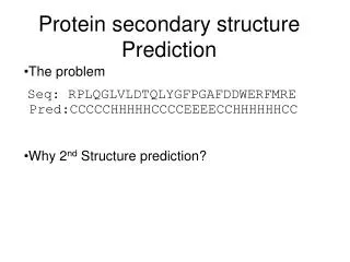
Assignment and prediction. Protein Secondary Structures. Helix. Bend. Turn. Secondary Structure Elements. ß-strand. * H = alpha helix * G = 3 10 - helix * I = 5 helix (pi helix) * E = extended strand, participates in beta ladder * B = residue in isolated beta-bridge

E N D
Assignment and prediction Protein Secondary Structures
Helix Bend Turn Secondary Structure Elements ß-strand
* H = alpha helix * G = 310 - helix * I = 5 helix (pi helix) * E = extended strand, participates in beta ladder * B = residue in isolated beta-bridge * T = hydrogen bonded turn * S = bend * C = coil Secondary Structure Type Descriptions
Classification of secondary structure • Defining features • Dihedral angles • Hydrogen bonds • Geometry • Assigned manually by crystallographers or • Automatic • DSSP (Kabsch & Sander,1983) • STRIDE (Frishman & Argos, 1995) • DSSPcont (Andersen et al., 2002)
Automatic assignment programs • DSSP ( http://www.cmbi.kun.nl/gv/dssp/ ) • STRIDE ( http://www.hgmp.mrc.ac.uk/Registered/Option/stride.html ) • DSSPcont ( http://cubic.bioc.columbia.edu/services/DSSPcont/ ) # RESIDUE AA STRUCTURE BP1 BP2 ACC N-H-->O O-->H-N N-H-->O O-->H-N TCO KAPPA ALPHA PHI PSI X-CA Y-CA Z-CA 1 4 A E 0 0 205 0, 0.0 2,-0.3 0, 0.0 0, 0.0 0.000 360.0 360.0 360.0 113.5 5.7 42.2 25.1 2 5 A H - 0 0 127 2, 0.0 2,-0.4 21, 0.0 21, 0.0 -0.987 360.0-152.8-149.1 154.0 9.4 41.3 24.7 3 6 A V - 0 0 66 -2,-0.3 21,-2.6 2, 0.0 2,-0.5 -0.995 4.6-170.2-134.3 126.3 11.5 38.4 23.5 4 7 A I E -A 23 0A 106 -2,-0.4 2,-0.4 19,-0.2 19,-0.2 -0.976 13.9-170.8-114.8 126.6 15.0 37.6 24.5 5 8 A I E -A 22 0A 74 17,-2.8 17,-2.8 -2,-0.5 2,-0.9 -0.972 20.8-158.4-125.4 129.1 16.6 34.9 22.4 6 9 A Q E -A 21 0A 86 -2,-0.4 2,-0.4 15,-0.2 15,-0.2 -0.910 29.5-170.4 -98.9 106.4 19.9 33.0 23.0 7 10 A A E +A 20 0A 18 13,-2.5 13,-2.5 -2,-0.9 2,-0.3 -0.852 11.5 172.8-108.1 141.7 20.7 31.8 19.5 8 11 A E E +A 19 0A 63 -2,-0.4 2,-0.3 11,-0.2 11,-0.2 -0.933 4.4 175.4-139.1 156.9 23.4 29.4 18.4 9 12 A F E -A 18 0A 31 9,-1.5 9,-1.8 -2,-0.3 2,-0.4 -0.967 13.3-160.9-160.6 151.3 24.4 27.6 15.3 10 13 A Y E -A 17 0A 36 -2,-0.3 2,-0.4 7,-0.2 7,-0.2 -0.994 16.5-156.0-136.8 132.1 27.2 25.3 14.1 11 14 A L E >> -A 16 0A 24 5,-3.2 4,-1.7 -2,-0.4 5,-1.3 -0.929 11.7-122.6-120.0 133.5 28.0 24.8 10.4 12 15 A N T 45S+ 0 0 54 -2,-0.4 -2, 0.0 2,-0.2 0, 0.0 -0.884 84.3 9.0-113.8 150.9 29.7 22.0 8.6 13 16 A P T 45S+ 0 0 114 0, 0.0 -1,-0.2 0, 0.0 -2, 0.0 -0.963 125.4 60.5 -86.5 8.5 32.0 21.6 6.8 14 17 A D T 45S- 0 0 66 2,-0.1 -2,-0.2 1,-0.1 3,-0.1 0.752 89.3-146.2 -64.6 -23.0 33.0 25.2 7.6 15 18 A Q T <5 + 0 0 132 -4,-1.7 2,-0.3 1,-0.2 -3,-0.2 0.936 51.1 134.1 52.9 50.0 33.3 24.2 11.2 16 19 A S E < +A 11 0A 44 -5,-1.3 -5,-3.2 2, 0.0 2,-0.3 -0.877 28.9 174.9-124.8 156.8 32.1 27.7 12.3 17 20 A G E -A 10 0A 28 -2,-0.3 2,-0.3 -7,-0.2 -7,-0.2 -0.893 15.9-146.5-151.0-178.9 29.6 28.7 14.8 18 21 A E E -A 9 0A 14 -9,-1.8 -9,-1.5 -2,-0.3 2,-0.4 -0.979 5.0-169.6-158.6 146.0 28.0 31.5 16.7 19 22 A F E +A 8 0A 3 12,-0.4 12,-2.3 -2,-0.3 2,-0.3 -0.982 27.8 149.2-139.1 120.3 26.5 32.2 20.1 20 23 A M E -AB 7 30A 0 -13,-2.5 -13,-2.5 -2,-0.4 2,-0.4 -0.983 39.7-127.8-152.1 161.6 24.5 35.4 20.6 21 24 A F E -AB 6 29A 45 8,-2.4 7,-2.9 -2,-0.3 8,-1.0 -0.934 23.9-164.1-112.5 137.7 21.7 37.0 22.6 22 25 A D E -AB 5 27A 6 -17,-2.8 -17,-2.8 -2,-0.4 2,-0.5 -0.948 6.9-165.0-123.7 138.3 18.9 38.9 20.8 23 26 A F E > S-AB 4 26A 76 3,-3.5 3,-2.1 -2,-0.4 -19,-0.2 -0.947 78.4 -27.2-127.3 111.5 16.4 41.3 22.3 24 27 A D T 3 S- 0 0 74 -21,-2.6 -20,-0.1 -2,-0.5 -1,-0.1 0.904 128.9 -46.6 50.4 45.0 13.4 42.1 20.2 25 28 A G T 3 S+ 0 0 20 -22,-0.3 2,-0.4 1,-0.2 -1,-0.3 0.291 118.8 109.3 84.7 -11.1 15.4 41.4 17.0 26 29 A D E < S-B 23 0A 114 -3,-2.1 -3,-3.5 109, 0.0 2,-0.3 -0.822 71.8-114.7-103.1 140.3 18.4 43.4 18.1 27 30 A E E -B 22 0A 8 -2,-0.4 -5,-0.3 -5,-0.2 3,-0.1 -0.525 24.9-177.7 -74.1 127.5 21.8 41.8 19.1 DSSP
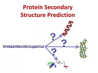
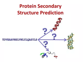
Prediction of protein secondary structure • What to predict? • How to predict? • How good are the best?
H E C Secondary Structure Prediction • What to predict? • All 8 types or pool types into groups DSSP * H = alpha helix * G = 310 -helix * I = 5 helix (pi helix) * E = extended strand * B = beta-bridge * T = hydrogen bonded turn * S = bend * C = coil
H E C Secondary Structure Prediction • What to predict? • All 8 types or pool types into groups Straight HEC * H = alpha helix * E = extended strand * T = hydrogen bonded turn * S = bend * C = coil * G = 310-helix * I = 5 helix (pi helix) * B = beta-bridge
Secondary Structure Prediction • Simple alignments • Align to a close homolog for which the structure has been experimentally solved. • Heuristic Methods (e.g., Chou-Fasman, 1974) • Apply scores for each amino acid an sum up over a window. • Neural Networks (different inputs) • Raw Sequence (late 80’s) • Blosum matrix (e.g., PhD, early 90’s) • Position specific alignment profiles (e.g., PsiPred, late 90’s) • Multiple networks balloting, probability conversion, output expansion (Petersen et al., 2000).
HoMo 1D ….the art of being humble FoRc The pessimistic point of viewPrediction by alignment
Secondary structure predictions of 1. and 2. generation • single residues (1. generation) • Chou-Fasman, GOR 1957-70/8050-55% accuracy • segments (2. generation) • GORIII 1986-9255-60% accuracy • problems • < 100% they said: 65% max • < 40% they said: strand non-local • short segments
1974 Chou & Fasman ~50-53% 1978 Garnier 63% 1987 Zvelebil 66% 1988 Quian & Sejnowski 64.3% 1993 Rost & Sander 70.8-72.0% 1997 Frishman & Argos <75% 1999 Cuff & Barton 72.9% 1999 Jones 76.5% 2000 Petersen et al. 77.9% Improvement of accuracy
Simple Alignments • Solved structure of a homolog to query is needed • Homologous proteins have ~88% identical (3 state) secondary structure • If no close homologue can be identified alignments will give almost random results
Name P(a) P(b) P(turn) f(i) f(i+1) f(i+2) f(i+3) Ala 142 83 66 0.06 0.076 0.035 0.058 Arg 98 93 95 0.070 0.106 0.099 0.085 Asp 101 54 146 0.147 0.110 0.179 0.081 Asn 67 89 156 0.161 0.083 0.191 0.091 Cys 70 119 119 0.149 0.050 0.117 0.128 Glu 151 37 74 0.056 0.060 0.077 0.064 Gln 111 110 98 0.074 0.098 0.037 0.098 Gly 57 75 156 0.102 0.085 0.190 0.152 His 100 87 95 0.140 0.047 0.093 0.054 Ile 108 160 47 0.043 0.034 0.013 0.056 Leu 121 130 59 0.061 0.025 0.036 0.070 Lys 114 74 101 0.055 0.115 0.072 0.095 Met 145 105 60 0.068 0.082 0.014 0.055 Phe 113 138 60 0.059 0.041 0.065 0.065 Pro 57 55 152 0.102 0.301 0.034 0.068 Ser 77 75 143 0.120 0.139 0.125 0.106 Thr 83 119 96 0.086 0.108 0.065 0.079 Trp 108 137 96 0.077 0.013 0.064 0.167 Tyr 69 147 114 0.082 0.065 0.114 0.125 Val 106 170 50 0.062 0.048 0.028 0.053 Chou-Fasman
Chou-Fasman 1. Assign all of the residues in the peptide the appropriate set of parameters. 2. Scan through the peptide and identify regions where 4 out of 6 contiguous residues have P(a-helix) > 100. That region is declared an alpha-helix. Extend the helix in both directions until a set of four contiguous residues that have an average P(a-helix) < 100 is reached. That is declared the end of the helix. If the segment defined by this procedure is longer than 5 residues and the average P(a-helix) > P(b-sheet) for that segment, the segment can be assigned as a helix. 3. Repeat this procedure to locate all of the helical regions in the sequence. 4. Scan through the peptide and identify a region where 3 out of 5 of the residues have a value of P(b-sheet) > 100. That region is declared as a beta-sheet. Extend the sheet in both directions until a set of four contiguous residues that have an average P(b-sheet) < 100 is reached. That is declared the end of the beta-sheet. Any segment of the region located by this procedure is assigned as a beta-sheet if the average P(b-sheet) > 105 and the average P(b-sheet) > P(a-helix) for that region. 5. Any region containing overlapping alpha-helical and beta-sheet assignments are taken to be helical if the average P(a-helix) > P(b-sheet) for that region. It is a beta sheet if the average P(b-sheet) > P(a-helix) for that region. 6. To identify a bend at residue number j, calculate the following value: p(t) = f(j)f(j+1)f(j+2)f(j+3) where the f(j+1) value for the j+1 residue is used, the f(j+2) value for the j+2 residue is used and the f(j+3) value for the j+3 residue is used. If: (1) p(t) > 0.000075; (2) the average value for P(turn) > 1.00 in the tetra-peptide; and (3) the averages for the tetra-peptide obey the inequality P(a-helix) < P(turn) > P(b-sheet), then a beta-turn is predicted at that location.
Chou-Fasman • General applicable • Works for sequences with no solved homologs • But the accuracy is low! • 50%
1974 Chou & Fasman ~50-53% 1978 Garnier 63% 1987 Zvelebil 66% 1988 Quian & Sejnowski 64.3% 1993 Rost & Sander 70.8-72.0% 1997 Frishman & Argos <75% 1999 Cuff & Barton 72.9% 1999 Jones 76.5% 2000 Petersen et al. 77.9% Improvement of accuracy
PHD method (Rost and Sander) • Combine neural networks with sequence profiles • 6-8 Percentage points increase in prediction accuracy over standard neural networks (63% -> 71%) • Use second layer “Structure to structure” network to filter predictions • Jury of predictors • Set up as mail server
Neural Networks • Benefits • General applicable • Can capture higher order correlations • Inputs other than sequence information • Drawbacks • Needs many data (different solved structures). • However, these does exist today (nearly 2500 solved structures with low sequence identity/high resolution.) • Complex method with several pitfalls
How is it done • One network (SEQ2STR) takes sequence (profiles) as input and predicts secondary structure • Cannot deal with SS elements i.e. helices are normally formed by at least 5 consecutive aminoacids • Second network (STR2STR) takes predictions of first network and predicts secondary structure • Can correct for errors in SS elements, i.e remove single helix prediction, mixture of strand and helix predictions
Weights Input Layer I K H E Output Layer E E C H V I I Q A E Hidden Layer Window IKEEHVIIQAEFYLNPDQSGEF….. Architecture
Weights Input Layer H E H C Output Layer E H C E C H E C Window Hidden Layer IKEEHVIIQAEFYLNPDQSGEF….. Secondary networks(Structure-to-Structure)
Example PITKEVEVEYLLRRLEE (Sequence) HHHHHHHHHHHHTGGG. (DSSP) ECCCHEEHHHHHHHCCC (SEQ2STR) CCCCHHHHHHHHHHCCC (STR2STR)
Prediction accuracy PHD Slide courtesy by B. Rost 2004
PSI-Pred (Jones) • Use alignments from iterative sequence searches (PSI-Blast) as input to a neural network (Just like PHDsec) • Better predictions due to better sequence profiles • Available as stand alone program and via the web
Petersen et al. 2000 • SEQ2STR (>70 networks) • Not one single network architecture is best for all sequences • STR2STR (>70 network) • => 4900 network predictions, • (wisdom of the crowd!!!) • Others have 1
Prediction accuracy (Q3=81.2%). 2006. (Petersen et al. 2000)
Spectrin homology domain (SH3) CEEEEEEECCCCCCCCCCCCCCCCEEEEEECCCCCEEEEEECCCEEEECCCCCEECC .EEEEESS.B...STTB..B.TT.EEEEEE..SSSEEEEEETTEEEEEEGGGEEE.. Petersen 93%
Benchmarking secondary structure predictions • CASP • Critical Assessment of Structure Predictions • Sequences from about-to-be-deposited-structures are given to groups who submit their predictions before the structure is published • Every 2. year • EVA • Newly solved structures are send to prediction servers. • Every week
EVA results (Rost et al., 2001) • PROFphd 77.0% • PSIPRED 76.8% • SAM-T99sec 76.1% • SSpro 76.0% • Jpred2 75.5% • PHD 71.7% • Cubic.columbia.edu/eva
Petersen et al. Proteins 2000 EVA: secondary structure 76%
Prediction of protein secondary structure • 1980: 55% simple • 1990: 60% less simple • 1993: 70% evolution • 2000: 76% more evolution • 2006: 80% more evolution • what is the limit? • 88% for proteins of similar structure • 80% for 1/5th of proteins with families > 100 • missing through: better definition of secondary structure including long-range interactions • structural switches • chameleon / folding
Links to servers • Database of links http://mmtsb.scripps.edu/cgi bin/renderrelres?protmodel • ProfPHD http://www.predictprotein.org/ • PSIPRED http://bioinf.cs.ucl.ac.uk/psipred/ • JPred http://www.compbio.dundee.ac.uk/~www-jpred/
Conclusions • The big break through in SS prediction came due to sequence profiles • Rost et al. • Prediction of secondary structure has not changed in the last 5 years • More protein sequences => higher prediction accuracy • No new theoretical break through • Accuracy is close to 80% for globular proteins • If you need a secondary structure prediction use one of profile based: • ProfPHD, PSIPRED, and JPred • And not one of the older ones such as : • Chou-Fasman • Garnier