Characterizing the Physical Environment of Urban Centers in Rondônia with Landsat ETM+

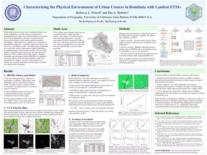
1. y = 0.868x + 7.96 R2 = 0.882 1:1 P232 R66 Modeled fraction Residual 2-emb 1 P231 emb1 + shade Vegetation R67 emb2 + shade ln(2000 Population) 3 Reference fraction Reference fraction 10 Impervious • • • 6 P230 3-emb 2 2 3 4 y = 0.747x + 5.56 R2 = 0.769 1:1 y = 1.11x + 7.39 R2 = 0.989 R68 + emb1 + emb2 shade Soil 7 5 + emb1 + emb3 4 shade 9 8 Modeled fraction • • • Residual Water ln(Area of Urban Extent) 4-emb + emb1 + emb2 emb3 + shade + + emb4 emb1 + emb2 shade Reference fraction Reference fraction • • • 0° Study site BR-364 Hwy Rondônia Major roads y = 0.805x + 3.23 R2 = 0.760 1:1 County seat Brasil Step 3 Apply simple SMA models Step 1 Data pre-processing Step 4 Select ‘best’ model for each pixel Step 5 Map V-I-S fractions for each pixel Landsat scene 0 50 100 200 Kilometers 0% 100% 0% 100% 0% 100% 0% 100% 0% 100% 0% 100% Modeled fraction 23.5°S Residual ETM+ image 2 3 4 • Convert to surface reflectance • Apply water mask Reference fraction Reference fraction Step 2 Build endmember library Reflectance image Image endmembers Step 6 Validate fractions Reference endmembers (a) (b) (a) (b) c. a. e. (c) (d) (c) (d) Table 3: Summary of accuracy assessment measures. If correlations were perfect, slope would equal 1 and intercept, 0. RSQ refers to the correlation coefficient; MAE refers to mean average error—the average absolute value of the difference between modeled and measured fraction values; bias refers to the average of the error; and RMSE refers to the root mean square error. b. f. d. Characterizing the Physical Environment of Urban Centers in Rondônia with Landsat ETM+ Rebecca L. Powell1 and Dar A. Roberts2 Department of Geography, University of California, Santa Barbara 93106-4060 U.S.A. 1becky@geog.ucsb.edu, 2dar@geog.ucsb.edu Methods Study Area Abstract While much effort has been devoted to studying rural land-cover change in Rondônia, very little work has considered the relationship between urban areas and regional land-cover change. A first step in building this connection is to characterize the physical environment of urban centers and their immediate surroundings. Urban land-cover is modeled as a combination of three primary components—vegetation, impervious surface, and soil (V-I-S)—in addition to water. Ten urban centers in Rondônia were selected for analysis, representing a range of populations, development histories, and economic activities. For each urban sample, a 20x20-km region centered over the built-up area was subset from 1999 or 2000 Landsat ETM+ imagery. Multiple endmember spectral mixture analysis (MESMA) was applied to each image subset, and the sub-pixel abundance of the V-I-S components was mapped. Accuracy of the modeled V-I-S fractions was assessed using high-resolution images mosaicked from digital aerial videography. The ten urban centers included in this study are presented in Figure 1 (right) and Table 1 (below). Our sample is somewhat biased to cities with larger populations, to include a large number of pixels dominated by built-up land cover. Sub-scenes centered on each study site, 20-km in each dimension, were extracted from the Landsat ETM+ scenes for further processing. Mapping urban environments is challenging because of their high spatial and spectral variability. We address these challenges as follows: • Spatial variability: Spectral mixture analysis (SMA) models each pixel as the linear sum of spectrally ‘pure’ endmembers • Spectral variability: Multiple endmember spectral mixture analysis (MESMA) allows the number and type of endmembers to vary on a per-pixel basis • The ‘best’ model for each pixel is the model that meets fractional constraints while minimizing RMS error. Figure 2 (at right) summarizes the methods applied to map the V-I-S components of urban land cover and surrounding landscape. Table 1: Study sites. ‘2000 Rank’ refers to the population rank out of 52 sedes de municípioin the state of Rondônia, based on the 2000 national census. Figure 2:Flowchart of methods, adapted from Rashed et al., 2003. Landsat ETM+ sub-scenes are converted to surface reflectance (Step 1), and a regionally specific spectral library is constructed (Step 2). All allowed SMA models are tested (Step 3), and the best model is selected for each pixel based on minimizing error (Step 4). An image of per-pixel fractional coverage for each V-I-S component is generated (Step 5), and accuracy is assessed by comparing the modeled fractions to fractional cover measured from classified aerial videography. Figure 1: Study area. Numbered study sites correspond with Table 1 (at left). Conclusions Results 1. MESMA Library and Models 3. Model Complexity Several potentially significant findings emerge from this analysis: • Modeled fractions and reference fractions are highly correlated, demonstrating the potential of moderate-resolution imagery to map the physical urban environment • Model complexity—how many endmembers are required to accurately model each pixel—is related to the degree of human impact on the landscape; highly impacted areas require more complex models • V-I-S components can capture inter- and intra-urban variability, suggesting that these data products can contribute to comparative studies of urbanizing areas Future directions will apply these techniques to a time series of data; for Rondônia, the archive of satellite imagery largely captures the timeline of urban development. We anticipate that comparing the evolution of urban across a region will serve as a valuable first step to build connections between social systems and the physical environment. Model complexity—how many endmembers are required to adequately model the materials in a pixel—was mapped for each sub-scene, resulting in several noticeable patterns: • Intact portions of the original landscape (e.g. primary forest and savanna) were dominated by 2-endmember models • Non-built-up, human-impacted portions of the landscape (e.g. pasture) were dominated by 3-endmember models • Built-up areas (e.g. urban centers and major roads) were dominated by 4-endmember models • The final endmember library contained 14 endmembers, in addition to photometric shade. Endmember spectra are presented in Figure 3 (right). Non-photosynthetic vegetation (NPV) was included as an additional class to account for senesced vegetation. • Allowed MESMA models consisted of all possible permutations of the generalized combinations listed in Table 2 (right). • Water pixels accounted for 0.4% of the total area. Almost 99.5% of non-water pixels were successfully modeled across all 10 sub-scenes. Figure 6: Complexity of the ‘best-fit’ model selected for each pixel. (a) Ji-Paraná and (b) Seringueiras (see Figures 4 and 5, respectively). Figure 3: (above) Spectral library selected for MESMA application. Table 2: (below) Allowed models by generalized material class, resulting in 14 two-endmember models, 76 three-endmember models, and 90 four-endmember models. We tested how well V-I-S characterization of urban environments captures the extent of built-up land cover using a well-established relationship between a city’s built-up area (A) and its population (P): A = aPb where constants a and b are empirically determined. Results are presented in Figure 7 (right) and indicate a very strong relationship (R2 = 0.989). 2. V-I-S Fraction Maps Maps of generalized fractions are shown for two samples below (Figures 4 and 5). Bright areas represent higher fractions, dark areas lower fractions, and black pixels indicate the absence of the material. The NPV (senesced vegetation) and green vegetation fractions were combined to generate the vegetation fraction map. Selected References Figure 7: Scatterplot of the natural log of urban extent, as delineated by four-endmember models, vs. the natural log of the 2000 urban population for the ten settlements included in the study. Dennison, P. E. & Roberts, D. A. (2003). Endmember selection for multiple endmember spectral mixture analysis using endmember average RMSE. Remote Sensing of Environment, 87, 123-135. Hess, L. L., Novo, E. M. L. M., et al. (2002). Geocoded digital videography for validation of land cover mapping in the Amazon basin. International Journal of Remote Sensing, 23, 1527-1556. IBGE (2000). Censo Demográfico. Rio de Janeiro, Brazil: Instituto Brasileiro de Geografia e Estatística. Powell, R. L., Matzke, N., et al. (2004). Sources of error in accuracy assessment of thematic land-cover maps in the Brazilian Amazon. Remote Sensing of Environment, 90, 221-234. Powell, R. L., Roberts, D. A., et al. (2005). Sub-pixel mapping of urban land cover using multiple endmember spectral mixture analysis: Manaus, Brazil. Remote Sensing of Environment, in review. Rashed, T., Weeks, J. R., et al. (2003). Measuring the physical composition of urban morphology using multiple endmember spectral mixture models. Photogrammetric Engineering and Remote Sensing, 69, 1011-1020. Roberts, D. A., Batista, G. T., et al. (1998). Change identification using multitemporal spectral mixture analysis: applications in Eastern Amazonia. In R. S. Lunetta and C. D. Elvidge (Eds), Remote Sensing Change Detection: Environmental Monitoring Methods and Applications (pp. 137-161). Chelsea, Michigan: Ann Arbor Press. Roberts, D. A., Gardner, M., et al. (1998). Mapping chaparral in the Santa Monica Mountains using multiple endmember spectral mixture models. Remote Sensing of Environment, 65, 267-279. 4. Accuracy Assessment • Reference data were produced from classified digital aerial videography, collected on June 22, 1999, as part of the Validation Overflights for Amazon Mosaics • Flight-lines intersected 3 urban areas in our sample: Ji-Paraná, Rolim de Moura, and Santa Luzia d’Oeste • Samples were selected from zoom videography (ground instantaneous field of view ~ 0.3 m) and compared to shade-normalized V-I-S fractions Figure 8: Comparisons between reference and modeled fractions: (a) Vegetation scatterplot, (b) Vegetation fraction residuals, (c) Impervious scatterplot, (d) Impervious fraction residuals, (e) Soil scatterplot, (f) Soil fraction residuals. Perfect agreement, represented by the 1:1 line, is displayed on the scatterplots. The ‘best-fit’ line is displayed on the residual plots to indicate general trends of over- and under-estimation. Figure 4: MESMA products for Ji-Paraná (sample 2, Table 1): (a) RGB composite of Landsat ETM+ bands 5,4,3; (b) Vegetation fraction, (c) Impervious fraction, (d) Soil fraction. Figure 5: MESMA products for Seringueiras (sample 9, Table 1): (a) RGB composite of Landsat ETM+ bands 5,4,3; (b) Vegetation fraction, (c) Impervious fraction, (d) Soil fraction. Acknowledgements: This research was funded in part by NASA-LBA Ecology and a NASA Earth System Science Graduate Student Fellowship.