Download
1 / 27
340 likes | 1.05k Views
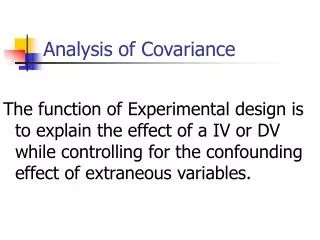
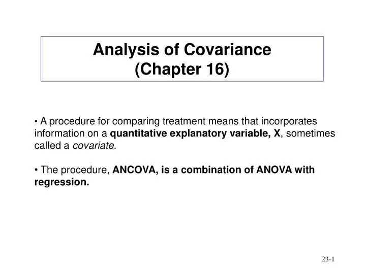
Analysis of Covariance (Chapter 16). A procedure for comparing treatment means that incorporates information on a quantitative explanatory variable, X , sometimes called a covariate . The procedure, ANCOVA, is a combination of ANOVA with regression. Example: Calf Weight Gain.

E N D
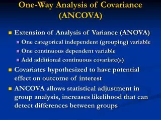
Analysis of Covariance(Chapter 16) • A procedure for comparing treatment means that incorporates information on a quantitative explanatory variable, X, sometimes called a covariate. • The procedure, ANCOVA, is a combination of ANOVA with regression.
Example: Calf Weight Gain • An animal scientist wishes to examine the impact of a pair of new dietary supplements on calf weight gain (response). • Three treatments are defined: standard diet, standard diet + supplement Q, and standard diet + supplement R. • All new calves from a large herd are available for use as study units. She selects 30 calves for study. Calves are randomized to the three diets at random (completely randomized design). • Initial weights are recorded, then calves are placed on the diets. At the end of four weeks the final weight is taken and weight gain is computed. • Simple analysis of variance and associated multiple comparisons procedures indicate no significant differences in weight gain between the two supplementary diets, but big differences between the supplemental diets and the standard diet. • Is this the end of the story? …
Simple ANOVA of a one-way classification would suggest no difference between Supplements Q and R but both different from Standard diet. ANOVA Results Average Weight Gain (Response g/day) xx x xx x x xx Standard Diet xxx xxx x xx + Supplement Q xx x x x xx x x x + Supplement R
Plotting of the initial weights by group shows that the groups were not equal when it came to initial weights. Initial Weights Initial Weight xx x x xx x x xx Standard Diet xx x xxxx x xx + Supplement Q x x x xx xx x x x + Supplement R
Weight Gain to Initial WeightStandard Diet Weight (kg) age If animals come into the study at different ages, they have different initial weights and are at different points on the growth curve. Expected weight gains will be different depending on age at entry into study.
Weight Gain (g/day) (Y) Initial Weight (x) Regression of Initial Weight to Weight Gain If we disregard the age of the animal but instead focus on the initial weight, we see that there is a linear relationship between initial weight and the weight gain expected.
Covariates Initial weight in the previous example is a covariable or covariate. A covariate is a disturbing variable (confounder), that is, it is known to have an effect on the response. Usually, the covariate can be measured but often we may not be able to control its effect through blocking. • In the EXAMPLE, had the animal scientist known that the calves were very variable in initial weight (or age), she could have: • Created blocks of 3 or 6 equal weight animals, and randomized treatments to calves within these blocks. • This would have entailed some cost in terms of time spent sorting the calves and then keeping track of block membership over the life of the study. • It was much easier to simply record the calf initial weight and then use analysis of covariance for the final analysis. • In many cases, due to the continuous nature of the covariate, blocking is just not feasible.
Expectations under Ho If all animals had come in with the same initial weight, All three treatments would produce the same weight gain. Under Ho: no treatment effects. Expected Weight Gain (g/day) (Y) Initial Weight (x) Average Weight Animal
Expectations under HA Under Ha: Significant Treatment effects + Supplement Q (q) + Supplement R (r) Standard Diet (c) WGQ WGR WGs Different treatments produce different weight gains for animals of the same initial weight. Expected Weight Gain (g/day) (Y) Initial Weight (x) Average Weight Animal
Different Initial Weights If the average initial weights in the treatment groups differ, the observed weight gains will be different, even if treatments have no effect. Under Ho: no treatment effects. WGR WGs WGQ Expected Weight Gain (g/day) (Y) cc c c cc c c cc qq q qqqq q qq r r r rr rr r r r Initial Weight (x)
Observed Responses under HA Suppose now that different supplements actually do increase weight gain. This translates to animals in different treatment groups following different, but parallel regression lines with initial weight. + Supplement Q + Supplement R r r r r Standard Diet r q r r r WGR r r q q q q WGQ q q c c q q c c c c q c WGs Under HA: Significant Treatment effects c c c Weight Gain (g/day) (Y) cc c c cc c c cc qq q qqqq q qq r r r rr rr r r r Initial Weight (x) What difference in weight gain is due to Initial weight and what is due to Treatment?
Simple one-way classification ANOVA (without accounting for initial weight) gives us the wrong answer! Observed Group Means Weight Gain (g/day) (Y) + Supplement Q + Supplement R r r r Standard Diet r r q r r r r r q q q q q q c c q q c q c c c c c c c cc c c cc c c cc qq q qqqq q qq r r r rr rr r r r Initial Weight (x) Unadjusted treatment means
Expected weight gain is computed for treatments for the average initial weight and comparisons are then made. Predicted Average Responses Weight Gain (g/day) (Y) + Supplement Q + Supplement R r r r Standard Diet r r q r r r r r q q q q q q c c q q c q c c c c c c c cc c c cc c c cc qq q qqqq q qq r r r rr rr r r r Initial Weight (x) Adjusted treatment means
ANCOVA: Objectives The objective of an analysis of covariance is to compare the treatment means after adjusting for differences among the treatments due to differences in the covariate levels for the treatments groups. The analysis proceeds by combining a regression model with an analysis of variance model.
Model The ai, i=1,…,t, are estimates of how each of the t treatments modifies the overall mean response. (The index j=1,…,n, runs over the n replicates for each treatment.) The slope coefficient, , is a measure of how the average response changes as the value of the covariate changes. The analysis proceeds by fitting a linear regression model with dummy variables to code for the different treatment levels.
A Priori Assumptions The covariate is related to the response, and can account for variation in the response. Check with a scatterplot of Y vs. X. The covariate is NOT related to the treatments. If Y is related to X, then the variance of the treatment differences is increased relative to that obtained from an ANOVA model without X, which results in a loss of precision. The treatment’s regression equations are linear in the covariate. Check with a scatterplot of Y vs. X, for each treatment. Non-linearity can be accommodated (e.g. polynomial terms, transforms), but analysis may be more complex. The regression lines for the different treatments are parallel. This means there is only one slope in the Y vs. X plots. Non-parallel lines can be accommodated, but this complicates the analysis since differences in treatments will now depend on the value of X.
Example • Four different formulations of an industrial glue are being tested. The tensile strength (response) of the glue is known to be related to the thickness as applied. Five observations on strength (Y) in pounds, and thickness (X) in 0.01 inches are made for each formulation. • Here: • There are t=4 treatments (formulations of glue). • Covariate X is thickness of applied glue. • Each treatment is replicated n=5 times at different values of X.
SAS Program data glue; input Formulation Strength Thickness; datalines; 1 46.5 13 1 45.9 14 1 49.8 12 1 46.1 12 1 44.3 14 2 48.7 12 2 49.0 10 2 50.1 11 2 48.5 12 2 45.2 14 3 46.3 15 3 47.1 14 3 48.9 11 3 48.2 11 3 50.3 10 4 44.7 16 4 43.0 15 4 51.0 10 4 48.1 12 4 46.8 11 ; run; procglm; class formulation; model strength = thickness formulation / solution ; lsmeans formulation / stderr pdiff; run; The basic model is a combination of regression and one-way classification.
Output: Use Type III SS to test significance of each variable MSE Source DF Squares Mean Square F Value Pr > F Model 4 66.31065753 16.57766438 10.17 0.0003 Error 15 24.44684247 1.62978950 Corrected Total 19 90.75750000 R-Square Coeff Var Root MSE Strength Mean 0.730636 2.691897 1.276632 47.42500 Source DF Type I SS Mean Square F Value Pr > F Thickness 1 63.50120135 63.50120135 38.96 <.0001 Formulation 3 2.80945618 0.93648539 0.57 0.6405 Source DF Type III SS Mean Square F Value Pr > F Thickness 1 53.20115753 53.20115753 32.64 <.0001 Formulation 3 2.80945618 0.93648539 0.57 0.6405 Standard Parameter Estimate Error t Value Pr > |t| Intercept 58.93698630 B 2.21321008 26.63 <.0001 Thickness -0.95445205 0.16705494 -5.71 <.0001 Formulation 1 -0.00910959 B 0.80810401 -0.01 0.9912 Formulation 2 0.62554795 B 0.82451389 0.76 0.4598 Formulation 3 0.86732877 B 0.81361075 1.07 0.3033 Formulation 4 0.00000000 B . . . Regression on thickness is significant. No formulation differences. Divide by MSE to get mean squares.
Least Squares Means(Adjusted Formulation means computed at the average value of Thickness [=12.45]) The GLM Procedure Least Squares Means Strength Standard LSMEAN Formulation LSMEAN Error Pr > |t| Number 1 47.0449486 0.5782732 <.0001 1 2 47.6796062 0.5811616 <.0001 2 3 47.9213870 0.5724527 <.0001 3 4 47.0540582 0.5739134 <.0001 4 Least Squares Means for effect Formulation Pr > |t| for H0: LSMean(i)=LSMean(j) Dependent Variable: Strength i/j 1 2 3 4 1 0.4574 0.3011 0.9912 2 0.4574 0.7695 0.4598 3 0.3011 0.7695 0.3033 4 0.9912 0.4598 0.3033
Formulation Strength Thickness 1 46.5 13 1 45.9 14 1 49.8 12 1 46.1 12 1 44.3 14 2 48.7 12 2 49.0 10 2 50.1 11 2 48.5 12 2 45.2 14 3 46.3 15 3 47.1 14 3 48.9 11 3 48.2 11 3 50.3 10 4 44.7 16 4 43.0 15 4 51.0 10 4 48.1 12 4 46.8 11 ANCOVA in Minitab Stat > ANOVA > General Linear Model … > Responses: Strength > Model: Formulation > Covariates: Thickness > Options: Adjusted (Type III) Sums of Squares General Linear Model: Strength versus Formulation Factor Type Levels Values Formulat fixed 4 1 2 3 4 Source DF Seq SS Adj SS Adj MS F P Thicknes 1 63.501 53.201 53.201 32.64 0.000 Formulat 3 2.809 2.809 0.936 0.57 0.640 Error 15 24.447 24.447 1.630 Total 19 90.758 Term Coef SE Coef T P Constant 59.308 2.099 28.25 0.000 Thicknes -0.9545 0.1671 -5.71 0.000 Formulat 1 -0.3801 0.5029 -0.76 0.462 2 0.2546 0.5062 0.50 0.622 3 0.4964 0.4962 1.00 0.333
ANCOVA in R > glue <- read.table("glue.txt",header=TRUE) > glue$Formulation <- as.factor(glue$Formulation) > # fit linear models: full, thickness only, formulation only > full.lm <- lm(Strength ~ Formulation + Thickness, data=glue) > thick.lm <- lm(Strength ~ Thickness, data=glue) > formu.lm <- lm(Strength ~ Formulation, data=glue) > > anova(thick.lm,full.lm) Analysis of Variance Table Model 1: Strength ~ Thickness Model 2: Strength ~ Formulation + Thickness Res.Df RSS Df Sum of Sq F Pr(>F) 1 18 27.2563 2 15 24.4468 3 2.8095 0.5746 0.6405 > anova(formu.lm,full.lm) Analysis of Variance Table Model 1: Strength ~ Formulation Model 2: Strength ~ Formulation + Thickness Res.Df RSS Df Sum of Sq F Pr(>F) 1 16 77.648 2 15 24.447 1 53.201 32.643 4.105e-05 *** Test for Formulation differences Test for significance of Thickness
> summary(full.lm) Call: lm(formula = Strength ~ Formulation + Thickness, data = glue) Residuals: Min 1Q Median 3Q Max -1.6380 -1.0398 0.1873 0.6966 2.3255 Coefficients: Estimate Std. Error t value Pr(>|t|) (Intercept) 58.92788 2.24551 26.243 5.97e-14 *** Formulation2 0.63466 0.83193 0.763 0.457 Formulation3 0.87644 0.81840 1.071 0.301 Formulation4 0.00911 0.80810 0.011 0.991 Thickness -0.95445 0.16706 -5.713 4.11e-05 *** > summary(thick.lm) Call: lm(formula = Strength ~ Thickness, data = glue) Residuals: Min 1Q Median 3Q Max -2.0813 -0.7324 0.1274 0.9090 1.9230 Coefficients: Estimate Std. Error t value Pr(>|t|) (Intercept) 59.9294 1.9504 30.726 < 2e-16 *** Thickness -1.0044 0.1551 -6.476 4.32e-06 *** Residual standard error: 1.231 on 18 degrees of freedom Multiple R-Squared: 0.6997, Adjusted R-squared: 0.683 F-statistic: 41.94 on 1 and 18 DF, p-value: 4.317e-06 R Full model (can be refined by omitting formulation) Reduced model (formulation omitted)
Plot lines for full model; but these can all be replaced by single line for reduced model (blue). R