Download
1 / 18
180 likes | 571 Views
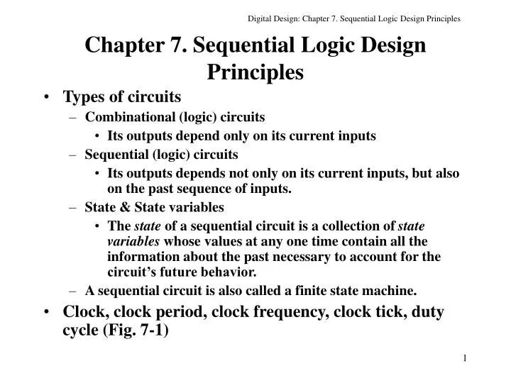
Chapter 7. Sequential Logic Design Principles. Types of circuits Combinational (logic) circuits Its outputs depend only on its current inputs Sequential (logic) circuits Its outputs depends not only on its current inputs, but also on the past sequence of inputs. State & State variables

E N D
Chapter 7. Sequential Logic Design Principles • Types of circuits • Combinational (logic) circuits • Its outputs depend only on its current inputs • Sequential (logic) circuits • Its outputs depends not only on its current inputs, but also on the past sequence of inputs. • State & State variables • The state of a sequential circuit is a collection of state variables whose values at any one time contain all the information about the past necessary to account for the circuit’s future behavior. • A sequential circuit is also called a finite state machine. • Clock, clock period, clock frequency, clock tick, duty cycle (Fig. 7-1)
7.1 Bistable Elements • Bistable element (Fig. 7-2) • Digital analysis (Fig. 7-2) • Analog analysis (Fig. 7-3) • Metastable (Fig. 7-4)
7.2 Latches and Flip-Flops • Flip-flop • A sequential device normally samples its inputs and changes its output only at times determined by a clocking signal. • Latch • A sequential device normally watches all of its inputs continuously and changes its output only at any time, independent of a clocking signal. • S-R latch (Fig. 7-5, 7-6, 7-7, 7-8) • S*-R* Latch (Fig. 7-9) • S-R latch with enable (Fig. 7-10, 7-11) • D latch (transparent latch) (Fig. 7-12, 7-13, 7-14)
Setup time (tsetup) • The setup time of a latch or a flip-flop is the time period before the clock arrival time that the data must arrive before that period such that the data can be stored safely into the latch or flip-flop. • Hold time (thold) • The hold time of a latch or a flip-flop is the time period after the clock arrival time that the data must hold its value such that the data can be stored into the latch or flip-flop. • Data should not be changed during setup and hold time period. • Edge-triggered D flip-flop (Fig. 7-15, 7-16, 7-17, 7-18) • master, slave, dynamic input indicator • Positive edge-triggered versus negative edge-triggered • Edge-triggered D flip-flop with asynchronous preset and preset (Fig. 7-19, Fig 7-20)
Edge-triggered D flip-flop with enable (Fig. 7-21) • Scan flip-flop (Fig. 7-22, 7-23) • Test-enable input, test input • Scan chain • Edge-triggered J-K flip-flop (Fig. 7-28, 7-29, 7-30) • T flip-flop (Fig. 7-32, 7-33, 7-34)
7.3 Clocked Synchronous State-Machine Analysis • A clocked synchronous state machine (Fig. 7-35) • State memory: a set of n flip-flops that store current state of the machine, and it has 2n distinct states. The flip-flops are synchronized by clock ticks. • Next state = F(current state, input) • Output = G(current state, input) • Mealy machine (Fig. 7-35) • Moore machine (Fig. 7-36) • Output is only a function of current state. • Mealy machine with pipelined outputs (Fig. 7-37) • Characteristic equations (Table 7-1) • Specify the flip-flop’s next state as a function of its current state and inputs
7.3.4 Analysis of State Machines with D Flip-Flops • Goal: To determine the next state and output functions so that the behavior of a circuit can be predicted. • Three basic steps • Determine the next-state and output functions F and G. • Use F and G to construct a state/output table. • Draw a state diagram. • Mealy machine example (Fig. 7-38): step-by-step • Excitation signals: D0 and D1 are inputs to the state memory. • Excitation Equations: Express the excitation signals as functions of the current state and inputs. D0=Q0 EN’ + Q0’ EN D1=Q1 EN’ + Q1’ Q0 EN + Q1 Q0’ EN
Employ characteristic equation of flip-flops Q0*=D0 and Q1*=D1 • Find Transition equations Q0*=Q0 EN’ +Q0’ EN Q1*=Q1 EN’ + Q1’ Q0 EN + Q1 Q0’ EN • Create Transition table use transition equation (Table 7-2) • Create State table by state assignment • Create State/output table use output equation MAX = Q1 Q0 EN • Draw State diagram (Fig. 7-39) • Moore machine example (Table 7-3, Fig. 7-40) • MAXS= Q1 Q0 • Yet another example (Fig. 7-43, Table 7-4, Fig. 7-44)
7.4 Clocked Synchronous State-machine Design • The steps for designing a clocked synchronous state machine are just about reverse of the analysis steps. • Construct a state/output table • State minimization (Optional) • State assignment: assign state variables to the named states • Create transition/output table • Choose flip-flop type • Construct an excitation table • Derive excitation equation • Derive output equation • Draw a logic diagram
State-table design example • Problem description: Design a clocked synchronous state machine with two inputs, A and B, and a single output Z that is 1 if: • A had the same value at each of the previous clock ticks, or • B has been 1 since the last time that the first condition was true. Otherwise, the output should be 0. • Timing diagram for example state machine (Fig. 7-47) • Design steps • Evolution of a state table (Fig. 7-48, Fig. 7-49) • State sequence for example state machine (Fig. 7-50) • State minimization (Fig. 7-51) • State and output table (Table 7-6)
State assignment (Table 7-7) • Choose an initial coded state into which the machine can easily be forced at reset (00…00 or 11…11). • Minimize the number of state variables that change on each transition. • …. • Unused states • Minimal risk: Make every unused states explicitly go to the known states, ex. Initial state. • Minimal cost:Treat the next states as don’t-care states. This is to assume that the machine never goes to unused states. • Synthesis using D flip-flops • Create a transition/output table (Table 7-8) • Create excitation/output table (table 7-9)
Draw excitation map (Minimal risk, Fig. 7-52) D1 = Q1 + Q2’ Q3’ D2 = Q1 Q3’ A’ + Q1 Q3 A + Q1 Q2 B D3 = Q1 A + Q2’ Q3’ A Z = Q1 Q2 Q3’ + Q1 Q2 Q3 = Q1 Q2 • Draw excitation map (Minimal cost, Fig. 7-53, Fig. 7-54) D1= 1 D2 = Q1 Q3’ A’ + Q3 A + Q2 B D3 = A Z = Q2
Another example (1s-counting machine) • Problem description • Design a clocked synchronous state machine with two inputs, X and Y, and one output , Z. The output should be 1 if the number of 1 inputs on X and Y since reset is a multiple of 4, and 0 otherwise. • Design steps • State and output table (Table 7-12) • Transition/excitation and output table (Table 7-13) • Excitation map (Fig. 7-57) • Excitation and output equation D1= Q2 X’ Y + Q1’ X Y + Q1 X’ Y’ + Q2 X Y’ D2= Q1’ X’ Y + Q1’ X Y’ + Q2 X’ Y’ + Q2’ X Y Z= Q1’ Q2’
Yet another example (Combination lock) • Problem description Design a clocked synchronous state machine with one input, X and two outputs, UNLK and HINT. The UNLK output should be 1 if and only if X is 0 and the sequence of inputs received on X at the preceding seven clock ticks was 0110111. The HINT output should be 1 if and only if the current value of X is the correct one to move the machine closer to being in the “unlocked” state (with UNLK=1). • Design steps • State and output table (Table 7-14) • Transition/excitation table (Table 7-15) • Excitation map for D flip-flops (Fig. 7-58) D1= Q1 Q2’ X + Q1’ Q2 Q3 X’ + Q1 Q2 Q3’ D2= Q2’ Q3 X + Q2 Q3’ X D3=Q1 Q2’ Q3’ + Q1 Q3 X’ + Q2’ X’ + Q3’ Q1’ X’ + Q2 Q3’ X
Output excitation map (Fig. 7-59) • UNLK= Q1 Q2 Q3 X’ • HINT= Q1’ Q2’ Q3’ X’ + Q1 Q2’ X + Q2’ Q3 X + Q2 Q3 X’ + Q2 Q3’ X
7.5 Designing State Machines Using State Diagrams • Difference between a state table and a state diagram • A state table is an exhaustive listing of the next states for each state/input combination. No ambiguity is possible. • A state diagram is a set of arcs labeled with transition expressions. Ambiguous state diagram is possible. • Example for state machine design using state diagram • Problem description • Tail light control of a 1965 Ford Thunderbird (Fig. 7-60, 7-61) • A Moore machine
Design steps • Initial state diagram and output table • Output equations LA= L1 + L2 + L3 + LR3 LB= L2 + L3 + LR3 LC = L3 + LR3 RA = R1 + R2 + R3 + LR3 RB = R2 + R3 + LR3 RC = R3 + LR3 • Check the ambiguity of a state diagram • Mutual exclusion • For each state, show that the logical product of each possible pair of transition expressions on arcs leaving that state is 0. • All inclusion • For each state, show that the logical sum of the transition expressions on all arcs leaving that state is 1.
A correct state diagram (Fig. 7-63) and an enhanced one (Fig. 7-64) • State assignment (Table 7-16) • Transition list (Table 7-17) • 7.11 ABEL Sequential-Circuit Design Features • 7.12 VHDL Sequential-Circuit Design Features