Download
1 / 49
570 likes | 1.13k Views
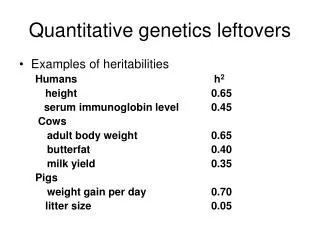
Quantitative Genetics Terminology: Qualitative traits – phenotypes differ by quality. Exp.: red/white eyes, wrinkled /round peas. Quantitative traits – phenotypes differ in quantity: height, yield, flower/fruit size, disease resistance

E N D
Quantitative Genetics Terminology: Qualitative traits – phenotypes differ by quality. Exp.: red/white eyes, wrinkled /round peas. Quantitative traits – phenotypes differ in quantity: height, yield, flower/fruit size, disease resistance Polygenic inheritance: more than one gene operating to make a single phenotype.
Phenotypes in qualitative inheritance are all distinct from each other - discontinuous variation. Traits in quantitative inheritance are not as easily categorized into distinct classes - continuous variation.
Quantitative Inheritance • Definition: when genes produce metrical effects of a trait of interest. • Quantitative traits display continuous variation; controlled by many genes, each with a small effect • Controlled by many segregating loci whose alleles affect the observed phenotype • However, both quantitative and qualitative traits follow the same laws of inheritance • e.g. dominance, epistasis, linkage, pleiotropism
General Considerations: • Normally assume genes are nuclear • Normally quantitative traits are more • affected by environmental effects • than are qualitative traits • Normally we see continuous variation; however, • continuity can be as much a consequence of • environmental influence as it is a • consequence of the number of segregating • loci.
Theoretical Distributions: No Dominance Dominance Theoretical distributions in F2. Model assumes: 1) 100% h2 2) 12 unit difference between P1 and P2 3) no linkage 4) dominance is isodirectional 75 50 25 0 75 50 25 0 1 gene 50 52 54 56 58 60 62 % Population 50 52 54 56 58 60 62 75 50 25 0 75 50 25 0 2 genes 50 52 54 56 58 60 62 50 52 54 56 58 60 62
Theoretical Distributions: No Dominance Dominance 45 30 15 0 45 30 15 0 6 genes As # of segregating loci increases; distribution is more ‘normal’ in appearance 50 52 54 56 58 60 62 % Population 50 52 54 56 58 60 62 30 25 20 15 10 5 0 30 25 20 15 10 5 0 12 genes 50 52 54 56 58 60 62 50 52 54 56 58 60 62
Gene action: As the number of loci controlling a trait increases, so do the number of genotypes and phenotypes When the loci produce a cumulative effect, the variation becomes continuous. Variation increases in a predictable manner
Example: If two gene pairs were involved, five F2 phenotypes in a 1:4:6:4:1 ratio would be expected.
A mathematical rule can be developed that relates the number of the phenotypes and the genes involved: Number of phenotypes = (# genes x 2) + 1 Or, you can predict the number of phenotypic classes by looking at the number of the genes operating (if it’s known) 2 genes yield 5 phenotypes 3 genes yield 7 phenotypes 4 genes yield 9 phenotypes
Number of genes involved in a quantitative inheritance can also be estimated using the equation: (P1-P2)2 N = 8(VF2 - VE)
Effect of the environment: Most quantitative traits are subject to environmental effects, which can cause individuals with same genotypes to have slightly different phenotypes.
History #1: Josef Kölreuter in early 19 century crossed tall and dwarf tobacco plants: F1: all intermediate in height; F2 showed continuous variation in height from tall to short Results supported biometricians theory that all traits were determined by many genes each having small effects
F2 phenotypes showed “normal distribution” or bell curve distribution.
History #2: • William Bateson (late 1800s - early 1900s): • ‘Mendelian’ • Multiple-factor or multiple-gene hypothesis (the earliest form of polygenic inheritance theory) • Quantitative traits were controlled by Mendelian ‘genes’. • Each genes contributes to the same phenotype • in a small but quantifiable way. i.e. Quantitative traits are controlled by multiple genes acting together
How to reconcile quantitative traits theory with Mendel’s theory? Nillson-Ehle (1909) made a cross between red-seeded wheat and white-seeded wheat: F1: All plants showed intermediate seed color. F2: continuous variation in kernel colors between red and white.
Among the continuous expression of colored grain phenotypes, about 1/64 showed completely white kernels (i.e. one of the parental phenotypes), and ~ 1/64 showed dark red kernels (i.e. the other parental phenotype)
1/64 matches the phenotype ratio produced by the combination of three recessive gene in a trihybrid cross. Conclusion: Quantitative inheritance also follows Mendel’s rule for inheritance; Wheat grain color is a quantitative trait governed by three pairs of genes.
The cross of white and red wheat involves three gene pairs: r1r1r2r2r3r3 x R1R1R2R2R3R3 The darkness of red color is proportional to the number of R. The darkest class, with 6 R alleles, shows the same color as the dark red parental and is one of two classes that breed true.
This means that the effect of allele R is additive – additive alleles effects are another feature of quantitative traits.
If the contribution of multiple genes to a quantitative trait is additive, then how do we estimate the contribution of each gene? For example: Plants with genotype as A1A1A1A1A1A1 produce 7 cm high progeny, while those with A2A2A2A2A2A2 produce 5 cm height. (Note: sometimes one of the extreme genotypes produces a base value or base line for the phenotype. In this example, there are no progeny with 0 cm height!)
How much does each allele contribute? Calculate difference between the two extremes: 7 – 5 = 2 cm 2) This difference is caused by 6 additive alleles; 3) Therefore, each additive allele causes an increase of 2/6 = 0.33 cm above the base height.
To predict the height of a plant with genotype A1A1A2A2A1A2: 5 + 3(0.33) = 5.99 cm height. But, don’t forget about the environmental effects…
Genetic Structure of a Population • Genetic structure • Self-pollinated vs. Cross-pollinated crops • Homozygous vs. Heterozygous • Homogeneous vs. Heterogeneous • Allele frequencies • H-W equilibrium • “Fixing” traits in a population
General Considerations • Self-pollinated crops • Heterogeneous population of homozygotes • Cross-pollinated crops • Heterogeneous population of heterozygotes
Changes in genotype and allele frequency • Plant breeding seeks to move the genetic composition of a population toward a predetermined end point • Accomplished through selection
Allelic Frequency • Genotype Frequency: proportion or % of individuals with a specific genotype Frequency AA AA AA AA f(AA)=1 AA AA AA AA AA AA AA AA
Allelic Statistics AAAaaa aa AA n1 + n2 + n3 = N AA aa AA D H R aa Aa Aa aa Aa Aa f(AA) = n1/N = D D+H+R=1 f(Aa) = n2/N = H f(aa) = n3/N = R
Hardy-Weinberg Law(1908) • Predicts probable genetic structure of a population • In it’s simplest form, the law states that 2 alleles, A and a, having frequencies p and q respectively, shall be represented in different genotypes with proportions equal to: p2 AA + 2pq Aa + q2 aa based on a specific set of assumptions
H-W Law Assumptions: • Population is infinitely large • Only random mating; no self-fertilization • No selective advantage (no selection) • No mutation, migration, or random genetic drift • No linkage
AA Aa aa p2 + 2pq + q2 Derivation of the H-W Equation p q A = p a = q a A AA Aa p A p2 pq Aa aa q a pq q2
Testing Equilibrium For allele A: D + 1/2H 2D + H or p = N 2N Where: p = Proportion or frequency of allele ‘A’ D = # of homozygous dominant individuals H = # of heterozygous individuals N = Total population
Testing Equilibrium For allele ‘a’: R + 1/2H 2R + H or q = N 2N Where: q = Proportion or frequency of allele ‘a’ R = # of Homozygous recessive individuals H = # of heterozygous individuals N = Total population
Allelic Statistics Gene Frequency (allele frequency) Genotype frequency in each population is determined by the allele frequency in the previous generation of the population In the absence of disruption, gene and genotype frequency will remain constant from generation to generation
Allele Frequency Calculation Example: ResistantModerate Susceptible Genotype AA Aa aa # 10 60 30 0.1 0.6 0.3 Genotypic freq (2x10)+60 = 0.4 f(A) = p = 100x2 p + q = 1 (2x30)+60 = 0.6 f(a) = q = 100x2
After 1 generation of H-W conditions Genotypic/Allelic frequency # 1: p2 + 2pq + q2 Where: D’, H’ and R’ represent the proportion in the new population AA D’ = (0.4)2 = 0.16 Aa H’ = 2 x 0.4 x 0.6 = 0.48 aa R’ = (0.6)2 = 0.36
After 1 generation of H-W conditions Genotypic/Allelic frequency # 2: p q a (.6) A (.4) AA Aa p A (.4) (.16) (.24) a (.6) Aa aa q (.24) (.36) In equilibrium: .16AA + .48Aa + .36aa = 1
Population not in H-W equilibrium: AAAaaa Obs # 40 80 80 f(A) =p = 0.4 Obs freq .2 .4 .4 f(a) =q = 0.6 Calc freq .16 .48 .36 Calc # 32 96 72 Test with Chi-square statistic: Test with 1 df because we lose 1 df to normal limitation and 1 df for using estimated ratio X2 = 5.56 w/1df; p< 0.05; reject Ho (pop not in HW eq)
Population not in H-W equilibrium will return to equilibrium after one generation of random mating .2 .4 .4 Aa AA aa AA x AA AA x Aa AA x aa AA .2 (.4)(.2)=.08 (.2)2=.04 (.2)(.4)=.08 Random mating = all possible combinations Aa x aa Aa x AA Aa x Aa Aa .4 .16 .16 .08 aa x Aa aa x aa aa x AA aa .4 .16 .16 .08
Can Summarize Crossings: MatingFreq ofProgeny matingAAAaaa 1 AAxAA 2 AAxAa 1 AaxAa 2 AAxaa 2 Aaxaa 1 aaxaa .04 .16 .16 .16 .32 .16 .04 .08 .08 .04 .08 .04 .16 .16 .16 .16 .16 .48 .36 w/in 1 generation Obs freq= calc freq
Population Statistics Effect of selection on allelic frequency: qo qn= 1+nqo Where: qn = allelic freq after nth generations qo = original allelic frequency n = number of generations
q1= 0.37 Example: changes in allelic frequency after 1 generation of selection away from susceptibility qo qn= 1+nqo Note: use allelic frequency of the allele selected against 0.6 q1= 1+(1*0.6) Therefore q = 0.37 and p (1-q) = 0.63 after one generation of selection
After 2 generations of selection against susceptibility: qo qn= 1+nqo 0.6 q2= After 3 generations: q3= 0.21 and p3= 0.79 1+ (2*0.6) q2= 0.27
Genotypic Frequency: Selection for Recessive Traits 1 generation to identify: F2AAAaaa 1/4 1/2 1/4 # Genes %F2 w/aa Minimum Pop Size 1 (1/4)1 or .25 10 2 (1/4)2 or .0625 46 3 (1/4)3 or .015 190 4 (1/4)4 or .004 765 n (1/4)n
Genotypic Frequency: Selection for Recessive Traits Minimum Population Size: ln (1-P) n= ln (1-p) So for aa: Where: n = population size P = probability p = freq of genotype ln (1-.95) n = ln (1-.25) n = approx 10 plants
Genotypic Frequency: Selection for Dominant Traits 2 generations to identify: F2AAAaaa Need to self A- and select non-segregating parents Progeny Test 1/4 1/2 1/4 3/4 So 3/4 can be divided into 1/3 AA and 2/3 Aa ln (1-.95) n = approx 7 plants n= ln (1-.33)