Download
1 / 57
590 likes | 712 Views
Finding the Molecular Basis of Quantitative Genetic Variation. Richard Mott Wellcome Trust Centre for Human Genetics Oxford UK. Genetic Traits. Quantitative (height, weight) Dichotomous (affected/unaffected) Factorial (blood group) Mendelian - controlled by single gene (cystic fibrosis)

E N D
Finding the Molecular Basis of Quantitative Genetic Variation Richard Mott Wellcome Trust Centre for Human Genetics Oxford UK
Genetic Traits • Quantitative (height, weight) • Dichotomous (affected/unaffected) • Factorial (blood group) • Mendelian - controlled by single gene (cystic fibrosis) • Complex – controlled by multiple genes*environment (diabetes, asthma)
Molecular Basis of Quantitative Traits QTL: Quantitative Trait Locus chromosome genes
Molecular Basis ofQuantitative Traits QTL: Quantitative Trait Locus chromosome QTG: Quantitative Trait Gene
Molecular Basis ofQuantitative Traits QTL: Quantitative Trait Locus chromosome SNP: Single Nucleotide Polymorphism QTG: Quantitative Trait Gene QTN: Quantitative Trait Nucleotide
Association Studies • Compare unrelated individuals from a population • Phenotypes: • Cases vs Controls • Quantitative measure • Genotypes: state of genome at multiple variable locations (Single Nucleotide Polymorphism = SNP) in each individual • Seek correlation between genotype and phenotype
Problems with Association Studies • Population stratification • Linkage Disequilibrium • Allele Frequencies • Multiple loci • Small Effect Sizes • Very few Successes
Population Stratification • If the sampling population comprises genetically distinct sub-populations with different disease prevalences • Then - • Any variant that distinguishes the sub-populations is likely to show disease association
Admixture Mapping • Population is homogeneous but each individual’s genome is a mosaic of segments from different populations • May be used to map disease loci • multiple sclerosis susceptibility • Reich et al 2005, Nature Genetics
Linkage Disequilibrium Mouse
Effects of Linkage Disequilibrium • Correlation between nearby SNPs • SNPs near to QTN will show association • Risk of false positive interpretation • But need only genotype “tagging” SNPs • ~ 1 million tagging SNPs will be in LD with ~50% of common variants in the human genome
The Common-Disease Common-Variant Hypothesis • Says • disease-predisposing variants will exist at relatively high frequency (i.e. >1%) in the population. • are ancient alleles occurring on specific haplotypes. • detectable in an case-control study using tagging SNPs. • Alternative hypothesis says • disease-predisposing alleles are sporadic new mutations, perhaps around the same genes, on different haplotypes. • families with history of the same disease owe their condition to different mutations events. • Theoretically detectable with family-based strategies which do not assume a common origin for the disease alleles, but are harder to detect with case-control studies (Pritchard, 2001).
Power Depends on • Disease-predisposing allele’s • Effect Size (Odds Ratio) • Allele frequency • Sample Size: #cases, #controls • Number of tagging SNPs • To detect an allele with odds ratio of 1.25 and with allele frequency > 1%, at 5% Bonferroni genome-wide significance and 80% power, we require • ~ 6000 cases, 6000 controls • ~ 0.5 million tagging SNPs, one of which must be in perfect LD with the causative variant • [Hirschorn and Daly 2005]
WTCCCWellcome Trust Case-Control Consortium • 2000 cases from each of • Type I Diabetes • Type II Diabetes • rheumatoid arthritis, • susceptibility to TB • bipolar depression • …. and others … • 3000 common controls • 0.675 million SNPs • ~10 billion genotypes • Data expected mid 2006
Disease studied directly Population and environment stratification Very many SNPs (1,000,000?) required Hard to detect trait loci – very large sample sizes required to detect loci of small effect (5,000-10,000) Potentially very high mapping resolution – single gene Very Expensive Animal Model required Population and environment controlled Fewer SNPs required (~100-10,000) Easy to detect QTL with ~500 animals Poorer mapping resolution – 1Mb (10 genes) Relatively inexpensive Map inHuman or Animal Models ?
QTL Mapping in Mice using Inbred Line Crosses • Genetically Homozygous – genome is fixed, breed true. • Standard Inbred Strains available • Haplotype diversity is controlled far more than in human association studies • QTL detection is very easy • QTL fine mapping is hard
Sizes of Mapped Behavioural QTL in rodents (% of total phenotypic variance)
QTL mapping: F2 Intercross X X A F1 B
QTL mapping: F2 Intercross X X A F1 F2 B
QTL mapping: F2 Intercross QTL +1 -1 0 0 0 +2 -2 F2 F1
QTL mapping: F2 Intercross +1 -1 0 0 0 +2 -2 F2 F1
QTL mapping: F2 Intercross Genotype a skeleton of markers across genome 20cM 0 0 +2 -2 F2
QTL mapping: F2 Intercross AB AA AB BA AB BA AB BA AB BA BA BA BA BA BA AA BA BA BA AA 0 0 +2 -2 BB BB AB AA F2
QTL mapping: F2 Intercross AB AA AB BA AB BA AB BA AB BA BA BA BA BA BA AA BA BA BA AA 0 0 +2 -2 BB BB AB AA F2
Single Marker Association • Test of association between genotype and trait at each marker position. • ANOVA • F2 crosses are • good for detecting QTL • bad for fine-mapping • typical mapping resolution 1/3 chromosome – 20-30 cM
Increasing mapping resolution • Increase number of recombinants: • more animals • more generations in cross
Heterogeneous Stocks • cross 8 inbred strains for >10 generations
Heterogeneous Stocks • cross 8 inbred strains for >10 generations
Heterogeneous Stocks • cross 8 inbred strains for >10 generations 0.25 cM
founders Mosaic Crosses G3 GN F20 inbreeding mixing chopping up HS, AI, outbreds F2, diallele RI (RIHS, CC)
Analysis of mosaic crosses chromosome markers • Want to predict ancestral strain from genotype • We know the alleles in the founder strains • Single marker association lacks power, can’t distinguish all strains • Multipoint analysis – combine data from neighbouring markers alleles 1 1 2 1 2 1 1 1 2 2 1 2 2 1 1 1 1 2 1 1 2 1 1 1 1 1 2 2 1 2 1 2 1 1
Analysis of mosaic crosses chromosome markers alleles 1 1 2 1 2 1 1 1 2 2 1 2 2 1 1 1 1 2 1 1 2 1 1 1 1 1 2 2 1 2 1 2 1 1 • Hidden Markov model HAPPY • Hidden states = ancestral strains • Observed states = genotypes • Unknown phase of genotypes • - analyse both chromosomes simultaneously • Output is probability that a locus is descended from a pair of strains • Mott et al 2000 PNAS
Testing for a QTL • piL(s,t) = Prob( animal i is descended from strains s,t at locus L) • piL(s,t) calculated using • genotype data • founder strains’ alleles • Phenotype is modelled yi = Ss,tpiL(s,t)T(s,t) + Covariatesi + ei • Test for no QTL at locus L • H0: T(s,t) are all same • ANOVA • partial F test
Example: Open Field Avtivity • Mouse Model for Anxiety
multipoint singlepoint significance threshold Talbot et al 1999, Mott et al 2000
Relation Between Marker and Genetic Effect QTL Marker 2 Marker 1 No effect observable Observable effect
Mapping Resolution in Mouse QTL experiments • F2 • ~25-50 Mb [250-300 genes] • HS • 1-5 Mb [10-50 genes] • Need More Resolution
Other Outbred Populations • Commercially available outbreds may contain more historical recombination • Potentially finer mapping resolution • How to exploit it ?