Download
1 / 27
270 likes | 276 Views
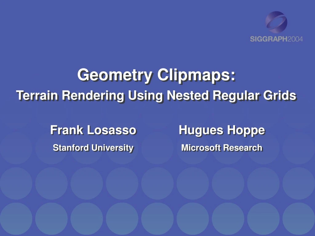
Geometry Clipmaps: Terrain Rendering Using Nested Regular Grids. Frank Losasso Stanford University. Hugues Hoppe Microsoft Research. Terrain Rendering Challenges. Mount Rainier. Concise storage No paging hick-ups Real-Time frame rates 60 fps Visual continuity No temporal pops.

E N D
Geometry Clipmaps:Terrain Rendering Using Nested Regular Grids Frank Losasso Stanford University Hugues Hoppe Microsoft Research
Terrain Rendering Challenges Mount Rainier • Concise storage No paging hick-ups • Real-Time frame rates 60 fps • Visual continuity No temporal pops Primary Dataset: United States at 30m spacing20 Billion samples Olympic Mountains
Previous Work • Irregular Meshes (e.g. [Hoppe 98]) • Fewest polygons • Extremely CPU intensive • Bin-trees (e.g. [Lindstrom et al 96]) • Simpler data structures / algorithms • Still CPU intensive • Bin-tree Regions (e.g. [Cignoni et al 03]) • Precomputed regions Decreased CPU cost • Temporal continuity difficult
Previous Work • Texture Clipmaps [Tanner 1998] • ‘Infinitely’ large textures • Clipped mipmap hierarchy • Modeling for the Plausible Emulation of Large Worlds [Dollins 2002] • Quadtree LOD around viewer • Terrain synthesis
Geometry Clipmaps • Store data in uniform 2D grids • Level-of-Detail from nesting of grids • Refine based on distance • Main Advantages • Simplicity • Compression • Synthesis
Terrain as a Pyramid • Terrain as mipmap pyramid • LOD using nested grids Coarsest Level Finest Level
Individual Clipmap Levels • Uniform 2D grid • Indexed triangle strip • Efficient caching • 60 M triangles/second • 255-by-255 grid • Expected Soon: • Vertex Textures
Inter-Level Transitions • Between respective power-of-2 grids
Inter-Level Transitions No transition Geometry transition Geometry & texture transition Gaps in geometry Gaps in texturing/shading
Inter-Level Transitions • Vertex shader blend geometry • Pixel shader blend textures • Both are inexpensive
Clipmap Update • For each level • Calculate new clipmap region • Fill new L-shaped region • Use toroidal arrays for efficiency
Clipmap Update • Update levels coarse-to-fine • Use limited update budget • Only render updated data • Fine levels may be cropped • Rendering load decreases as update load becomes to large for the budget
‘Filling’ New Regions • Two Sources: • Computed on-demand at 60 frames/second Decompressed explicit terrain Synthesized new terrain
Clipmap Update • Fine level from coarse level • U is a 16 point C1 smooth interpolant • For synthesized terrain, X =Gaussian noise • For explicit terrain, X = compression residual
Terrain Synthesis • Adds high frequency detail • Upsample then add Gaussian noise • Precomputed 50-by-50 noise texture • Per-octave amplitude from real terrain
Subdivision Interpolant Bilinear Interpolant (C0) 16-point Interpolant (C1)
Terrain Compression • Create mipmap fine-to-coarse • D found from data such that:
Terrain Compression • Calculate residuals coarse-to-fine • Upsample and compute inter-level residual • Quantize and compress residual • Replace approximation Prevent error accumulation
Compression Results • U.S height map • 30m horizontal spacing • 1m vertical resolution • 216,000-by-93,600 grid • 40GB uncompressed • 350MB compressed factor of over 100 • rms error 1.8m (6% of sample spacing)
Level-of-detail Error • Analyzed statistically See paper • For U.S. terrain (640-by-480 resolution) • rms error = 0.15 pixels • max error = 12 pixels • 99.9th percentile = 0.90 pixels
Graphics Hardware Friendly • Can be implemented in hardware • Clipmap levels as high-precision textures • Subdivision and normal calculation [Losasso et al 03] • Morphing already done in hardware • Noise from Noise() or from texture • Uploaded on-demand • Decompressed terrain
Limitations • Statistical error analysis • Assumes bounded spectral density • Unnecessarily many triangles • Assumes uniformly detailed terrain but, allows for optimal rendering throughput
Advantages • Simplicity • Optimal rendering throughput • Visual continuity • Steady rendering • Graceful degradation • Compression • Synthesis