Download
1 / 16
170 likes | 364 Views
Chapter 4. Discrete Probability Distributions Section 4.5: Geometric Distribution. Jiaping Wang Department of Mathematical Science 02/13/2013, Monday. Outline. Probability Function Mean and Variance An Alternative Parameterization Homework #5. Part 1. Probability Function.

E N D
Chapter 4. Discrete Probability DistributionsSection 4.5: Geometric Distribution Jiaping Wang Department of Mathematical Science 02/13/2013, Monday
Outline Probability Function Mean and Variance An Alternative Parameterization Homework #5
Suppose that a series of test firing of a rocket engine can be represented by a sequence of independent Bernoulli random variables with Yi=1 if ith trial is a success and Yi=0, otherwise. Assume the probability p of each trial is constant, denote X as the number of failures before the first success, then what is P(X=x)? P(X=x) = p(x) = P(Y1=0, Y2=0, …, Yx=0, Yx+1=1) = P(Y1=0)P(Y2=0)…P(Yx=0)P(Yx+1=1) = (1-p)(1-p)…(1-p)p = (1-p)xp=qxp, x= 0, 1, 2, …., q=1-p
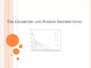
Probability Function The geometric distribution function: P(X=x)=p(x)=(1-p)xp=qxp, x= 0, 1, 2, …., q=1-p P(X=x) = qxp = p[qx-1p] = qP(X=x-1) <P(X=x-1) as q ≤ 1, for x=1, 2, … A Geometric Distribution Function with p=0.5
Example 4.15 A recruiting firm finds that 20% of the applicants for a particular sales position are fluent in both English and Spanish. Applicants are selected at random from the pool and interviewed sequentially. Find the probability that five applicants are interviewed before finding the first applicant who is fluent in both English and Spanish. Solution: X=5, p=0.2, using the geometric distribution function, we have P(X=5)=(0.8)5(0.2)=0.066
Geometric Series and CDF The geometric series: {tx: x=0, 1, 2, …} Sum of Geometric series: For |t|<1, we have = Sum of partial series: = Then we can verify The cumulative distribution function: F(x)=P(X≤x)===1-qx+1 And P(X≥x)=1-F(x-1)=qx
Mean and Variance The Expected Value E(X)= The Variance V(X)= E(X)= So E(X)/(pq) = And E(X)/p = [0 + q + 2q2 + … ] Thus, E(X)/(pq)-E(X)/p = 1+q+q2+q3+ • • • = 1/(1-q) E(X)=
Example 4.16 Referring to Example 4.15, let X be the number of unqualified applicants interviewed before the first qualified one. Suppose that the first applicant who is fluent in both English and Spanish is offered the position, and the applicant accepts. Suppose each interview costs $125. 1. Find the expected value and the variance of the total cost of interviewing until the job is filled. 2. Within what interval should this cost be expected to fall? As X+1 is the number of the trial on which the interviewing ends, so the total cost C=125(X+1)=125X + 125, thus E(C) = 125E(X)+125 = 125(0.8/0.2)+125=625, V(C)=1252V(X) =1252(0.8/0.04)=312500, the standard deviation is 559. By Chebysheff’s Inequality, the cost C will lie within two standard deviations of its mean at least 75% of the time, so the cost will be between 625-2(559) and 625+2(599).
Memoryless Property Memoryless Property means if we have observed j straight failures, then the probability of observing at least k more failures (at least j+kfailures in total) before a success is the same as if we were just beginning and wanted to determine the probability of observing at least k failures before the first success, that is: P(X ≥ j+k | X ≥ j) = P(X ≥ k). P(X≥ j+k|X ≥j)=
Example 4.17 Referring to Example 4.15, suppose that 10 applicants have been interviewed and no person fluent in both English and Spanish has been identified. What is the probability that 15 unqualified applicants will be interviewed before finding the first applicant who is fluent in English and Spanish? P(X=15|X≥10)= Which means the probability that 15 unqualified applicants will be interviewed before finding an applicant who is fluent in English and Spanish, given that the first 10 are not qualified, is equal to the probability of finding the first qualified candidate after interviewing 5 unqualified applicants.
The geometric distribution can serve as a model for a number of applications that are not associated with Bernoulli trials. Counting data, such as the number of insects on a plant or the number of weeds within a square foot area, may be well modeled by the geometric distribution.
Example 4.18 The number of weeds within a randomly selected square meter of a pasture has been found to be well modeled using the geometric distribution. For a given pasture, the number of weeds per square meter averages 0.5. What is the probability that no weeds will be found in a randomly selected square meter of this pasture? In this example, it doesn’t make sense to talk about Bernoulli trials and the probability of success. Instead, we have counts 0, 1, 2, … So let X denote the number of weeds in a randomly selected square meter of the pasture. We know E(X)=0.5 = (1-p)/p p=2/3, then we can find P(X=0)=p=2/3, so we can say there is a probability of (1-2/3) of seeing one or more weeds in a randomly selected square meter.
Homework #5 Page 134: 4.46, 4.48 Page 135: 4.52, 4.55 Page 136: 4.58 Page 150: 4.65