Download
1 / 37
370 likes | 488 Views
Preliminary comparison results of the October 2003 experiment with GroundWinds NH and NOAA's mini-MOPA lidar. S. Tucker 1,2 , I. Dors 3 , R. Michael Hardesty 1 , and Wm. Alan Brewer 1 Acknowledgements: A. Weickmann 1,2 and M. J. Post 4 ¹ Optical Remote Sensing Group

E N D
Preliminary comparison results of the October 2003 experiment with GroundWinds NH and NOAA's mini-MOPA lidar S. Tucker1,2, I. Dors3, R. Michael Hardesty1, and Wm. Alan Brewer1 Acknowledgements: A. Weickmann1,2 and M. J. Post4 ¹Optical Remote Sensing Group Chemical Sciences Division (CSD) Earth System Research Laboratory http://www.etl.noaa.gov/et2 ²Cooperative Institute for Research in Environmental Science University of Colorado, Boulder, CO ³University of New Hampshire, 4Zel Technologies, LLC/NOAA, Working Group on Space-Based Lidar Winds Key West, FL, January 17-20, 2005
October 2003 Field Experiment • NOAA’s mini-MOPA Coherent DWL • GroundWinds New Hampshire DWL • Occasional balloon-sonde launches NOAA’s 2005 Comparison and Validation Objectives Use analysis and comparisons to mini-MOPA data to: • Verify GWNH performance • Ability to accurately measure wind profiles • Precision & accuracy (in stares and profiles) • Check for improvements over GWNH 2000 data • Verify photon count – extend to technological scaling to space. • Quantify sensitivity improvements due to Photon Recycling
Additional Activities: Mini-MOPA Analysis Take advantage of long stare times in windy climate to study: • Sensitivity versus theoretical limit of the instrument • Effect of pulse duration on sensitivity • Extraction of mini-MOPA data at low SNR in the free troposphere • Pulse modeling • Turbulence profiling
Zeroth lag estimation: Mayor, et. al., J. Atmos. Oceanic Tech, 1997 Spectral noise floor estimation Spectrum at 1.26 km range Spectrum at range 0 10 2 gate mean floor spectral amplitude 0 0.2 0.4 0.6 0.8 1 1.2 1.4 1.6 1.8 2 Autocovariance function at 1.26 km Range Frequency (Hz) 0.11 N lag ACF linear fit ACF 0.1 autocorrelation 0.09 0.08 0 1 2 3 4 5 6 7 8 9 10 lags Velocity Variance Estimation Methods • Brovko-Zrnic Cramer-Rao Lower Bound: Rye & Hardesty, IEEE Trans Geoscience & Remote Sensing,1993. • UNH method: Standard deviation of 1 minute sliding window (5-6 samples at 10 s averaging times)
0 0.5 1 1.5 Alt. km MOPA s vs. wbSNR. GW031025_0336, File 8. v 1 ACF lin fit Ideal CRLB 0.8 0.6 (m/s) v 0.4 s 0.2 0 -12 -10 -8 -6 -4 -2 0 2 4 Wide-band SNR (dB) Mini-MOPA: Sensitivity versus theoretical limit of the instrument • CNR dependent-minimum standard deviation values calculated using the linear fit to 0th lag of the ACF • Black line: BZ-CRLB for these CNR values • Square fill colors represent altitude according to the colorbar. • Room for improvement? • CRLB: Rye & Hardesty, IEEE Trans Geoscience & Remote Sensing,1993.
Gaussian 1 m s m MOPA 1 s 0 0.5 1 1.5 Alt. km MOPA s vs. wbSNR. GW031025_0336, File 8. v 1 ACF lin fit Ideal CRLB 0.8 0.6 (m/s) v 0.4 s 0.2 0 -12 -10 -8 -6 -4 -2 0 2 4 Wide-band SNR (dB) Mini-MOPA pulses: effect on velocity variance 1 Autocovariance Function 0.8 0.6 MOPA xcov Pulse Shape 0.4 0.2 0 0 2 4 6 8 10 Lags
NOAA’s GWNH Validation Activities and mini-MOPA comparisons • Verify MOPA’s usefulness as a comparison measurement • Independent estimation of GWNH velocity variance • Range-independent variation removal • Photon-recycling vs. no Photon-recycling • Comparison between GWNH and NOAA’s mini-MOPA lidar • Comparison of wind measurements • Comparison of turbulence measurements • Characterization of measurement biases • Characterization of systematic effects • Comparison of boundary layer performance LWG – Key West, FL January 17-20, 2005
10/31/03MOPA & Balloon-Sonde 10/31/03MOPA & Balloon-Sonde 6 6 MOPA profile:3:27:43 Balloon D200310310722.MWO MOPA 5 5 4 4 Altitude (km) 3 3 2 2 1 1 Balloon MOPA 0 0 0 10 20 30 250 300 350 Wind Speed (m/s) Wind Direction (deg.) Mini-MOPA wind profile validation
Removal of GWNH offsets affecting all range gates (to improve precision estimates) • Take signal at each range gate & find linear trend. • Remove linear trend – left with variations about that trend. • Average the variations (not applicable in cases of strong turbulence)
GW Variance estimates (photon recycled data) σv estimates match UNH supplied measurement limit at altitudes above 6.5 km – Instrument/Camera limitations dominate Difference between UNH’s measurement limit and photon limit is described in UNH reports. sub 6.5 km results –Instrument and camera limitations cease to dominate. Other limitations? UNH supplied Meas. Limit Ö BW/ (NPED) Standard Deviation vs. Altitude NH_20031025051258_M57 16 15 14 13 12 11 10 9 8 Altitude (km) 7 CSD-corrected linear fit ACF 6 Uncorrected - linear fit ACF 5 CSD-corrected Spectral noise floor Uncorrected - Spectral noise floor 4 CSD-corrected 1 min std Uncorrected 1 min std (UNH method). 3 2 1 0 0 1 2 3 4 5 6 7 8 9 10 11 12 13 14 15 s (m/s) v
CSD-corrected linear fit ACF Uncorrected - linear fit ACF CSD-corrected Spectral noise floor Uncorrected - Spectral noise floor CSD-corrected 1 min std Uncorrected 1 min std. UNH supplied Meas. Limit Ö BW/ (NPED) Standard Deviation vs. Altitude NH_20031025051258_M57 9 GW Variance estimates post-correction (PR) • Uncorrected σv estimates: ACF and Spectral methods more optimistic then 1 minute σv estimates. • Post-correction σv estimates match UNH supplied measurement limit down to ~ 2km • Near 2 km altitude errors due to presence of thin clouds. 8 7 6 5 Altitude (km) 4 3 2 1 0 0 0.5 1 1.5 2 2.5 s (m/s) v
(post-correction) σv Ratios Spectral noise floor ratio th ACF 0 lag est. ratio Measurement limit ratio s 1 minute ratio v Ö 1/ (PED ratio) th linear fit 0 lag ACF th linear fit 0 lag ACF PR UNH Meas. Lim UNH Meas. Lim PR BW/ (NPED) Ö BW/ (NPED(PR)) Ö PHOTON RECYCLING: σv Ratios • Photon count ratios of ~2, ideally correspond to σv ratios of ~0.71. • Ratio of Photon Recycling (PR) to non PR σv estimates vary around the ratios of UNH supplied measurement limits (usually 0.75 to 0.9) • See UNH report regarding PR “quality factor” Standard Deviation vs. Altitude NH_20031025051258_M57 10 9 8 7 6 Altitude (km) 5 4 3 2 1 0 0 0.5 1 1.5 2 2.5 3 s (m/s) v
10/31/03, GWNH with Photon Recycling 20031031034030_M110 8 GWNH profile:03:40:30 7 MOPA profile:3:27:43 D200310310722.MWO 6 5 Altitude (m) 4 3 2 Balloon 1 MOPA GWNH-A GWNH-M 0 0 10 20 30 Wind Speed (m/s) Wind Profile Comparisons
Wind Profile Comparisons Altitude (km) Altitude (km) Altitude (km)
° ° ° ° Az =180 , GW Time:231.3 Az =225 , GW Time:251.6 Az =270 , GW Time:271.7 Az =315 , GW Time:287 MOPA profile:231.7 MOPA profile:252 MOPA profile:270.8 MOPA profile:286 6 6 6 6 5 5 5 5 4 4 4 4 Altitude (km) 3 3 3 3 2 2 2 2 1 1 1 1 0 0 0 0 -10 -5 0 5 -5 0 5 10 15 20 0 10 20 30 0 5 10 15 20 25 V (m/s) V (m/s) V (m/s) V (m/s) est est est est ° ° ° Az =0 , GW Time:302.4 Az =45 , GW Time:316.7 Az =90 , GW Time:331 MOPA profile:303.1 MOPA profile:315 MOPA profile:323.3 6 6 6 Molecular Molecular PR 5 5 5 balloon MOPA projected 4 4 4 MOPA Direct Altitude (km) 3 3 3 2 2 2 1 1 1 0 0 0 -10 -5 0 5 10 -15 -10 -5 0 5 10 -20 -10 0 10 V (m/s) V (m/s) V (m/s) est est est Single Az. Profile Comparisons for Molecular Channel
Summary • Mini-MOPA performance is as modeled. MOPA data provides useful comparisons for low-level GW data. • GWNH wind profiles generally compare well to those of MOPA and balloon-sonde data when clouds are not present. • GWNH velocity variations approach the measurement limit modeled by UNH, however they are significantly higher than the theoretical detected-photon limit. • UNH has attributed this degradation in velocity-variation, relative to the photon-limit, to receiver limitations. • GWNH measurements show variable offsets relative to mini-MOPA and balloon-sonde data.
Assorted References • B. J. Rye, “Estimate optimization parameters for incoherent backscatter heterodyne lidar including unknown signal bandwidth,” Appl. Opt., 39, 6086-6096 (2000). • B. J. Rye, “Comparative precision of distributed backscatter Doppler lidars,” Appl. Opt. 34, 8341-8344 (1995). • R. Frehlich, “Estimation of Velocity Error for Doppler Lidar Measurements,” J. Atmos. Oceanic. Tech, 18, 2001, 1628-1639. • D. H. Lenschow, V. Wulfmeyer, and C. Senff, “Measuring Second- through Fourth-order Moments in Noisy Data,” J. of Atmos. Ocean. Tech., 17, 1330-1347, (2000). • S. D. Mayor, D. H. Lenschow, R. L. Schwiesow, J. Mann, C. L. Frush, and M. K. Simon, “Validation of NCAR 10.6-m CO2 Doppler Lidar Radial Velocity Measurements and Comparison with a 915-MHz Profiler,” J. Atmos. Oceanic Tech., 14, 1997, 1110-1126. • B. J. Rye, R. M. Hardesty, “Discrete Spectral Peak Estimation in Incoherent Backscatter Heterodyne Lidar. I: Spectral Accumulation and the Cramer-Rao Lower Bound,” IEEE Trans Geoscience & Remote Sensing, 31, 1993, pp 16-27. LWG – Key West, FL January 17-20, 2005
° ° ° ° Az =180 , GW Time:231.3 Az =225 , GW Time:251.6 Az =270 , GW Time:271.7 Az =315 , GW Time:287 MOPA profile:231.7 MOPA profile:252 MOPA profile:270.8 MOPA profile:286 6 6 6 6 5 5 5 5 4 4 4 4 Altitude (km) 3 3 3 3 2 2 2 2 1 1 1 1 0 0 0 0 -10 -5 0 5 -5 0 5 10 15 20 0 10 20 30 0 5 10 15 20 25 HV (m/s) V (m/s) V (m/s) V (m/s) est est est est ° ° ° Az =0 , GW Time:302.4 Az =45 , GW Time:316.7 Az =90 , GW Time:331 MOPA profile:303.1 MOPA profile:315 MOPA profile:323.3 6 6 6 Aerosol Aerosol PR 5 5 5 balloon MOPA projected 4 4 4 MOPA Direct Altitude (km) 3 3 3 2 2 2 1 1 1 0 0 0 -10 -5 0 5 10 -15 -10 -5 0 5 10 -20 -10 0 10 V (m/s) V (m/s) V (m/s) est est est Single Az. Profile Comparisons for Aerosol Channel
10/31/03, GWNH without Photon Recycling 10/31/03, GWNH with Photon Recycling 20031031034030_M110 20031031034030_M110 8 8 GWNH profile:03:40:30 GWNH profile:03:40:30 7 7 MOPA profile:3:27:43 MOPA profile:3:27:43 D200310310722.MWO D200310310722.MWO 6 6 5 5 Altitude (m) Altitude (m) 4 4 3 3 2 2 Balloon Balloon 1 1 MOPA MOPA GWNH-A GWNH-A GWNH-M GWNH-M 0 0 0 5 10 15 20 25 30 0 5 10 15 20 25 30 Wind Speed (m/s) Wind Speed (m/s)
10/31/03, GWNH without Photon Recycling 10/31/03, GWNH with Photon Recycling 20031031034030_M110 20031031034030_M110 8 8 Balloon Balloon MOPA MOPA GWNH-A 7 GWNH-A 7 GWNH-M GWNH-M 6 6 GWNH profile:03:40:30 GWNH profile:03:40:30 5 MOPA profile:3:27:43 MOPA profile:3:27:43 5 D200310310722.MWO D200310310722.MWO 4 4 3 3 2 2 1 1 0 240 260 280 300 320 340 0 240 260 280 300 320 340 Wind Direction (deg.) Wind Direction (deg.)
GWNH Validation Activities GroundWinds • Sensitivity versus theoretical limit of the instrument for NH and HA systems • Sensitivity improvements made at GWNH since the LidarFest. • Total system transmission and recycling efficiencies • Technological scaling to potential airborne and space systems • Comparison of performance between the New Hampshire and Hawaii systems LWG – Key West, FL January 17-20, 2005
0 -5 Velocity Estimate (m/s) -10 -15 0.2 0.4 0.6 0.8 1 Pulse Width ( m s) Decreasing Pulse Width: Increased velocity variance & offset Inconsistent CRLB fits and velocity offsets led to further investigation of the MOPA pulse formation process…
AOM2 -44 MHz AOM1 +54 MHz FFT FFT output from AOMs 12 Pass Lorentzian Gain, |H(ω)| H(ω) 1.5 1 normalized gain 0.5 6 Pass 0 3.2068 3.2068 3.2069 3.2069 H(ω) frequency 13 x 10 Lorentzian Phase output from amplifiers 20 Line center Pulse center normalized phase 0 -20 3.2068 3.2068 3.2069 3.2069 frequency 13 x 10 Mini-MOPA Pulse Formation: Block Diagram ω0 CW CO2 Laser RF Discharge Optical Amplifiers
1 0.8 10 MHz 0.6 Normalized Amplitude 1 μs pulse 0.4 0.2 0 frequency 1 0.8 500 ns pulse 0.6 Normalized Amplitude 0.4 0.2 0 frequency 1 1 0.8 0.8 1 μs pulse Δf=0.1Mhz=-0.5m/s 0.6 0.6 Normalized Amplitude Normalized Amplitude 0.4 0.4 500 ns pulse Δf=0.55Mhz=-2.5m/s 0.2 0.2 0 0 frequency frequency Mini-MOPA pulse modeling Exaggerated examples of asymmetric effect on velocity estimates
1 0.8 0.6 MOPA xcov 0.4 m MOPA 1 s m Gaussian 1 s 0.2 MOPA 500 ns 0 0.5 1 1.5 Alt. Gaussian 500 ns 0 km 0 2 4 6 8 10 Lags MOPA s vs. wbSNR. GW031025_0336, File 8. v 1 1.6 m MOPA 1 s ACF lin fit m Gaussian 1 s 1.4 Ideal CRLB MOPA 500 ns 0.8 1.2 Gaussian 500 ns 1 0.6 CRLB (m/s) 0.8 v 0.4 0.6 s 0.4 0.2 0.2 0 0 -10 -5 0 5 10 15 20 -12 -10 -8 -6 -4 -2 0 2 4 CNR (dB) Wide-band SNR (dB) Mini-MOPA pulses: effect on velocity variance ACF CRLB Model with pulses at 10 MHz off amplifier line-center
3 2 60 m pulse, vertical stare velocity estimates 1 2 range (km) 0 -1 1 -2 Mini-MOPA: Velocity Offset vs. Pulse Width 0 -1 -2 -3 Velocity Estimate (m/s) -4 Average frequency monitor velocity estimate vs. pulse width -5 -6 0.3 0.4 0.5 0.6 0.7 0.8 0.9 1 Pulse Width (μs)