Feature Extraction

1. Feature Extraction Dmitry Chirkin, LBNL IceCube Collaboration meeting in Berkeley, March 2005

2. What is Feature Extraction • Given an ATWD or FADC waveform, determine arrival times of all photons which contributed: • hit series • FEInfo: combination or leading edge, width, charge (or amplitude) • Also applicable to AMANDA TWR

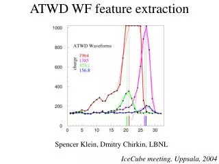
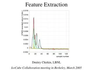
3. Feature Extraction last fall (DFL data) Fitted function: p0+A0 exp(-(t-t0)/s0)(1-exp(-(t-t0)2/s02))

4. undershooting: 1 mV for 50 mV pulse (Christopher Wendt): +~(exp(-(t-t0)/dt)-1) • possible extra late pulse (PMT anode configuration artifact) (Shigeru Yoshida) fit independetly • pedestal drift (corrected for by the fat-reader) New “features” discovered since

5. find first peak using the existing algorithm (refined with the root fit) • construct difference with the fitted function, weight by 1/F(waveform) to emphasize all peaks (big and small) • find maximum and add SPE fit function with t0 close to it Multi-peak fit

6. Multi-peak fit (cont.) • Fit the sum of two SPE functions to the waveform • repeat for all SPE terms with amplitude above the threshold until the quality of the fit stops improving

7. In-Ice Fits (low PEs)

8. In-Ice Fits (high PEs)

9. IceTop Fits

10. Other feature extraction “features” • other fitting functions were tried: log-normal (by Tom McCauley)  provides a different description of the rising leading edge • the undershooting is now fitted, so higher ATWD channels should be used not only for saturated values, but also for values close to 0 • zero-suppression road grader algorithm needs be modified to suppress the “most-repeated value” instead of 0 • the higher ATWD channels are narrower, creating extra “mismatch” peak at the trailing edge. •  higher-channel peaks need to be widened before they are combined with channel 0

11. Other feature extraction “features” • a “slewing” correction (shift of the leading edge proportional to width) may need to be made to the leading edge to describe electronics delays • Laser DFL or flasher in-ice calibration? • another correction proportional to high-voltage needs must made to describe high-voltage-dependent delay of the developing signal in the PMT •  Laser DFL calibration should be sufficient?

12. IceTray FE implementation • FeatureExtractor is a project on glacier, a part of: • OFFLINE-SOFTWARE • FATDATA •  example script is in the fat-reader/resources/ directory •  you can control: • MaxNumHits: maximum number of separate SPE functions to be fit, if necessary (default 20) • through the “DataOptions” of the fat-reader select hits that only pass a certain fraction of SPE threshold (--thrs) • At this time hidden in the source code: • maximum SPE waveform width – reduce it to split up large pulses into smaller ones (default 6 bins) • fixed parameters for the description of undershooting

13. FeatureExtractor usage and dataclasses • ATWDChannelMerger must be plugged in to produce the CombinedATWD waveform used by the FeatureExtractor • I3DOMCalibration class was modified to accommodate calibration and combining of the ATWD channels of different size: •  now Set methods set by ATWD bin “name”, 0-127 in reversed time order, as before •  now Get methods get by the time-ordered ATWD bin number, 0-127 in correct time order  this changed •  need not worry about this if only combined ATWD traces or Feature-Extracted hits are used

14. Conclusions • possibility to fit multi-peak waveforms was a highly-anticipated feature, which should be considered a major improvement • precision of the multi-peak fits for complicated waveforms is proportional to the time one is willing to spend on extracting features from waveforms: from a few milliseconds for 2-3 peaks to a few seconds for 10 to a few dozen seconds for 20. • ATWDChannelMerger and I3DOMCalibration class were modified to accommodate for hits with different ATWD-channel sizes (e.g., currently for in-ice: 128, 32, 32) • FeatureExtractor is a part of both OFFLINE-SOTWARE, and FATDATA. For the FeatureExtractor development the FATDATA provides a more versatile environment, allowing for a fast selection of the high- or low-PE events.

15. Road-grader zero-suppression • Common SPE-like waveform: • pedestal is shifted down compared to the value expected from calibration. This is a well-known (by now) effect and is corrected by the fat-reader • ok to use road-grader as is

16. Road-grader zero-suppression • A large-amplitude, saturated waveform: • undershoot is not recorded by the current road-grader implementation, but is a part of the waveform “features”

17. Road-grader zero-suppression • Highly-saturated muti-PE waveform: • the undershooting and small pulses on top of the undershot tail are all suppressed by the road-grader. Both amount of the undershooting and small pulses are features of the waveform and are used/reconstructed by the FeatureExtractor

18. Road-grader proposed modifications • find the “most-repeated” value, and compress all values above and below it (no more than a threshold-setting away) • this requires one pass over the incoming waveform and a small (~256 byte) memory buffer • the zero-suppressed value itself should be encoded into the compressed data • to make word length more uniform (11 bits all the time), prepend the 10-bit number of the next zero-suppressed words with “1”, and all other (10-bit) values with “0”. This is more uniform (and possibly efficient) than the current road-grader + Huffman-encoding algorithm

19. Dawn’s MPE set Dawn’s SPE set Modified road-grader compression ratio