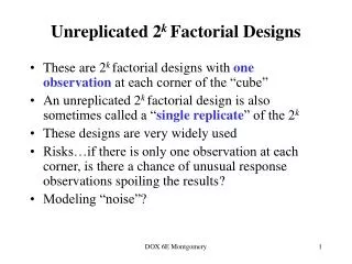
Download
1 / 24
240 likes | 381 Views
Follow-up Experiments to Remove Confounding Between Location and Dispersion Effects in Unreplicated Two-Level Factorial Designs. Andr é L. S. de Pinho *+ Harold J. Steudel * S øren Bisgaard # * Department of Industrial Engineering - University of Wisconsin-Madison

E N D
Follow-up Experiments to Remove Confounding Between Location and Dispersion Effects in Unreplicated Two-Level Factorial Designs André L. S. de Pinho*+ Harold J. Steudel* Søren Bisgaard# *Department of Industrial Engineering - University of Wisconsin-Madison +Department of Statistics - Federal University of Rio Grande do Norte (UFRN) - Brazil #Eugene M. Isenberg School of Management - University of Massachusetts, Amherst
Outline • Introduction • Motivation • Montgomery’s (1990) Injection Molding Experiment • Research Proposal • Current Research Results
Introduction • Motivation • Ferocious competition in the market • High pressure for lowering cost, shortening time-to-market and increase reliability • Need to have faster, better and cheaper processes • Current trend: Design for Six Sigma (DSS) • Approach: Robust product design • Making products robust to process variability • DOE provides the means to achieve this goal
Montgomery’s (1990) Injection Molding Experiment • fractional factorial design plus four center points with the objective of reducing the average parts shrinkage and also reducing the variability in shrinkage from run to run. • The factors studied • mold temperature (A), screw speed (B), holding time (C), gate size (D), cycle time (E), moisture content (F), and holding pressure (G). • The generators of the design were E = ABC, F = BCD, and G = ACD
Plausible Location Models Two possible location models: Montgomery’s Model (M1) = 27.3125 + 6.9375A + 17.8125B + 5.9375AB McGrath and Lin’s model (M2) = 27.3125 + 6.9375A + 17.8125B + 5.9375AB –2.6875CG – 2.4375G
Dispersion Effect Analysis Box and Meyer Dispersion Effect Statistics Dispersion effect
Conclusion Montgomery's Model (M1) = 27.3125 + 6.9375A + 17.8125B + 5.9375AB (dispersion effect in C) McGrath and Lin’s Model (M2) = 27.3125 + 6.9375A + 17.8125B + 5.9375AB –2.6875CG – 2.4375G (no dispersion effects [d.e.])
Minimum Number of Trials Montgomery’s (1990) injection molding • Addressed by McGrath (2001), 4 extra runs • The selection is done in such a way that A and B are fixed and each combination of the settings for columns 7 and 13 occurs • There are four sets of rows, (1, 5, 9, 13), (2, 6, 10, 14), (3, 7, 11, 15), and (4, 8, 12, 16). He selected (1, 5, 9, 13)
A B C G - - - - - - - - - - + - - + + + Minimum Number of Trials Graphical Representation 60, 52 R = 8 26, 27 R = 11 60, 60 R = 0 32, 34 R = 2 B Recommended runs for replication 4, 16 R = 12 15, 5 R = 10 C 6, 8 R = 2 10, 12 R = 2 A
1 - Bayesian method of finding active factors • in fractionated screening experiments • [Box and Meyer (1993)] • 2 - Apply a suitable transformation to ensure constant variance • 3 - Sequential design method for discrimination among concurrent models • [Box and Hill (1967)] Research Proposal • Expanding Meyer, Steinberg and Box (1996) to accommodate the presence of d.e. in the models
1 - Bayesian Method of Finding Active Factors Scenario • Fractionated Factorial Designs • Sparsity Principle Underlines the Process Being Studied • Allow the Inclusion of Non-Structured Models
Bayesian Method of Finding Active Factors Cont. Interpretation of the Posterior Probability The first one can be regarded as a penalty for increasing the number of variables in the model Mi. The second component is nothing less than a measure of fit
Finding Active Factors – Injection Molding Experiment Considering non-structured models Considering structured models Marginal Posterior Probabilities – Pj
Response M1 M2 X Two Rival Models Model Discrimination (MD) Criterion Overview Two Possible Models (M1) and (M2) to describe a Response
MD Criterion Cont. MD in the context of DOE: Remark:Must have constant variance for all models considered!
Outlines of the Transformation Procedure • Use WLS of the expanded location model is in the sense of the Bergman and Hynén (1997) method of identifying dispersion effects • Once we have available the residuals from the expanded location model we can then calculate the ratio,
Rearranged Covariance Matrix of Y } d (-) } Symmetric d (+)
Transformation – Injection Molding Experiment Montgomery’s (1990) Injection Molding Experiment (M1) = 27.3125 + 6.9375A + 17.8125B + 5.9375AB. (d.e. in C) (M2) = 27.3125 + 6.9375A + 17.8125B + 5.9375AB –2.6875CG – 2.4375G.(no d.e.) • The minimum number of trials to resolve the confounding problem is four • The possible sets of four runs that can be used for the follow-up experiment are (1, 5, 9, 13), (2, 6, 10, 14), (3, 7, 11, 15), and (4, 8, 12, 16) • McGrath then suggested (1, 5, 9, 13) for replication because it is near the optimum condition.
Finding the Expanded Model • The set of active location effects is L = {I, A, B, AB} • The set of dispersion effect is D = {C} • M1-expanded model is represented by the set = {I, A, B, C, AB, AC, BC, ABC} • (M1-expanded) = 27.3125 + 6.9375A + 17.8125B – 0.4375C + 5.9375AB – 0.8125AC – 0.9375BC + 0.1875ABC • The estimated weight is = 0.167
A B C G + + + + + + + + - - + - - + + + 60, 52 R = 8 26, 27 R = 11 60, 60 R = 0 32, 34 R = 2 B 4, 16 R = 12 15, 5 R = 10 Recommended runs for replication C 6, 8 R = 2 10, 12 R = 2 A MD Criterion – Injection Molding MD criterion and the design points Remark: McGrath’s suggestion, (1, 5, 9, 13), was the second-best discriminated follow-up design!
References • Bergman, B. and Hynén, A. (1997). “Dispersion Effects from Unreplicated Designs in the 2k-p Series”, Technometrics, 39, 2, 191-198. • Box, G. E. P. and Hill, W. J. (1967). “Discrimination Among Mechanistic Models”, Technometrics, 9, 1, 57-71. • Box, G. E. P. and Meyer, R. D. (1993). “Finding the Active Factors in Fractionated Screening Experiments”, Journal of Quality Technology, 25, 2, 94-105. • McGrath, R. N. (2001). “Unreplicated Fractional Factorials: Two Location Effects or One Dispersion Effect?”, Joint Statistical Meetings(JSM) in Atlanta. • Meyer, R. D., Steinberg, D. M., and Box, G. E. P. (1996). “Follow-up Designs to Resolve Confounding in Multifactor Experiments”, Technometrics, 38, 4, 303-313. • Montgomery, D. C. (1990). “Using Fractional Factorial Designs for Robust Process Development”, Quality Engineering, 3, 2, 193-205.