Download

1 / 50
520 likes | 540 Views
Introduction to Conjoint Analysis. Adapted from Sawtooth Software, Inc. materials. Different Perspectives, Different Goals. Buyers want all of the most desirable features at lowest possible price

E N D
Introduction to Conjoint Analysis Adapted from Sawtooth Software, Inc. materials
Different Perspectives, Different Goals • Buyers want all of the most desirable features at lowest possible price • Sellers want to maximize profits by:1) minimizing costs of providing features 2) providing products that offer greater overall value than the competition
Demand Side of Equation • Typical market research role is to focus first on demand side of the equation • After figuring out what buyers want, next assess whether it can be built/provided in a cost- effective manner
Products/Services are Composed of Features/Attributes • Credit Card:Brand + Interest Rate + Annual Fee + Credit Limit • On-Line Brokerage:Brand + Fee + Speed of Transaction + Reliability of Transaction + Research/Charting Options
Breaking the Problem Down • If we learn how buyers value the components of a product, we are in a better position to design those that improve profitability
How to Learn What Customers Want? • Ask Direct Questions about preference: • What brand do you prefer? • What Interest Rate would you like? • What Annual Fee would you like? • What Credit Limit would you like? • Answers often trivial and unenlightening (e.g. respondents prefer low fees to high fees, higher credit limits to low credit limits)
How to Learn What Is Important? • Ask Direct Questions about importances • How important is it that you get the <<brand, interest rate, annual fee, credit limit>> that you want?
Stated Importances • Importance Ratings often have low discrimination:
Stated Importances • Answers often have low discrimination, with most answers falling in “very important” categories • Answers sometimes useful for segmenting market, but still not as actionable as could be
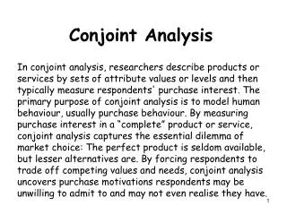
What is Conjoint Analysis? • Research technique developed in early 70s • Measures how buyers value components of a product/service bundle • Dictionary definition-- “Conjoint: Joined together, combined.” • Marketer’s catch-phrase-- “Features CONsidered JOINTly”
Important Early Articles • Luce, Duncan and John Tukey (1964), “Simultaneous Conjoint Measurement: A New Type of Fundamental Measurement,” Journal of Mathematical Psychology, 1, 1-27 • Green, Paul and Vithala Rao (1971), “Conjoint Measurement for Quantifying Judgmental Data,” Journal of Marketing Research, 8 (Aug), 355-363 • Johnson, Richard (1974), “Trade-off Analysis of Consumer Values,” Journal of Marketing Research, 11 (May), 121-127 • Green, Paul and V. Srinivasan (1978), “Conjoint Analysis in Marketing: New Development with Implications for Research and Practice,” Journal of Marketing, 54 (Oct), 3-19 • Louviere, Jordan and George Woodworth (1983), “Design and Analysis of Simulated Consumer Choice or Allocation Experiments,” Journal of Marketing Research, 20 (Nov), 350-367
How Does Conjoint Analysis Work? • We vary the product features (independent variables) to build many (usually 12 or more) product concepts • We ask respondents to rate/rank those product concepts (dependent variable) • Based on the respondents’ evaluations of the product concepts, we figure out how much unique value (utility) each of the features added • (Regress dependent variable on independent variables; betas equal part worth utilities.)
What’s So Good about Conjoint? • More realistic questions:Would you prefer . . .210 Horsepower or 140 Horsepower17 MPG 28 MPG • If choose left, you prefer Power. If choose right, you prefer Fuel Economy • Rather than ask directly whether you prefer Power over Fuel Economy, we present realistic tradeoff scenarios and infer preferences from your product choices
What’s So Good about Conjoint? • When respondents are forced to make difficult tradeoffs, we learn what they truly value
First Step: Create Attribute List • Attributes assumed to be independent (Brand, Speed, Color, Price, etc.) • Each attribute has varying degrees, or “levels” • Brand: Coke, Pepsi, Sprite • Speed: 5 pages per minute, 10 pages per minute • Color: Red, Blue, Green, Black • Each level is assumed to be mutually exclusive of the others (a product has one and only one level level of that attribute)
Rules for Formulating Attribute Levels • Levels are assumed to be mutually exclusiveAttribute: Add-on featureslevel 1: Sunrooflevel 2: GPS Systemlevel 3: Video Screen • If define levels in this way, you cannot determine the value of providing two or three of these features at the same time
Rules for Formulating Attribute Levels • Levels should have concrete/unambiguous meaning“Very expensive” vs. “Costs $575”“Weight: 5 to 7 kilos” vs. “Weight 6 kilos” • One description leaves meaning up to individual interpretation, while the other does not
Rules for Formulating Attribute Levels • Don’t include too many levels for any one attribute • The usual number is about 3 to 5 levels per attribute • The temptation (for example) is to include many, many levels of price, so we can estimate people’s preferences for each • But, you spread your precious observations across more parameters to be estimated, resulting in noisier (less precise) measurement of ALL price levels • Better approach usually is to interpolate between fewer more precisely measured levels for “not asked about” prices
Rules for Formulating Attribute Levels • Whenever possible, try to balance the number of levels across attributes • There is a well-known bias in conjoint analysis called the “Number of Levels Effect” • Holding all else constant, attributes defined on more levels than others will be biased upwards in importance • For example, price defined as ($10, $12, $14, $16, $18, $20) will receive higher relative importance than when defined as ($10, $15, $20) even though the same range was measured • The Number of Levels effect holds for quantitative (e.g. price, speed) and categorical (e.g. brand, color) attributes
Rules for Formulating Attribute Levels • Make sure levels from your attributes can combine freely with one another without resulting in utterly impossible combinations (very unlikely combinations OK) • Resist temptation to make attribute prohibitions (prohibiting levels from one attribute from occurring with levels from other attributes)! • Respondents can imagine many possibilities (and evaluate them consistently) that the study commissioner doesn’t plan to/can’t offer. By avoiding prohibitions, we usually improve the estimates of the combinations that we will actually focus on. • But, for advanced analysts, some prohibitions are OK, and even helpful
Conjoint Analysis Output • Utilities (part worths) • Importances • Market simulations
Conjoint Utilities (Part Worths) • Numeric values that reflect how desirable different features are:Feature UtilityVanilla 2.5Chocolate 1.825¢ 5.335¢ 3.250¢ 1.4 • The higher the utility, the better
Conjoint Importances • Measure of how much influence each attribute has on people’s choices • Best minus worst level of each attribute, percentaged:Vanilla - Chocolate (2.5 - 1.8) = 0.7 15.2%25¢ - 50¢ (5.3 - 1.4) = 3.9 84.8% ----- -------- Totals: 4.6 100.0% • Importances are directly affected by the range of levels you choose for each attribute
Market Simulations • Make competitive market scenarios and predict which products respondents would choose • Accumulate (aggregate) respondent predictions to make “Shares of Preference” (some refer to them as “market shares”)
Market Simulation Example • Predict market shares for 35¢ Vanilla cone vs. 25¢ Chocolate cone for Respondent #1:Vanilla (2.5) + 35¢ (3.2) = 5.7Chocolate (1.8) + 25¢ (5.3) = 7.1 • Respondent #1 “chooses” 25¢ Chocolate cone! • Repeat for rest of respondents. . .
Market Simulation Results • Predict responses for 500 respondents, and we might see “shares of preference” like: • 65% of respondents prefer the 25¢ Chocolate cone
Conjoint Market Simulation Assumptions • All attributes that affect buyer choices in the real world have been accounted for • Equal availability (distribution) • Respondents are aware of all products • Long-range equilibrium (equal time on market) • Equal effectiveness of sales force • No out-of-stock conditions
Shares of Preference Don’t Always Match Actual Market Shares • Conjoint simulator assumptions usually don’t hold true in the real world • But this doesn’t mean that conjoint simulators are not valuable! • Simulators turn esoteric “utilities” into concrete “shares” • Conjoint simulators predict respondents’ interest in products/services assuming a level playing field
Value of Conjoint Simulators… Some Examples • Lets you play “what-if” games to investigate value of modifications to an existing product • Lets you estimate how to design new product to maximize buyer interest at low manufacturing cost • Lets you investigate product line extensions: do we cannibalize our own share or take mostly from competitors? • Lets you estimate demand curves, and cross-elasticity curves • Can provide an important input into demand forecasting models
Three Main “Flavors” of Conjoint Analysis • Traditional Full-Profile Conjoint • Adaptive Conjoint Analysis (ACA) • Choice-Based Conjoint (CBC), also known as Discrete Choice Modeling (DCM)
Strengths of Traditional Conjoint • Good for both product design and pricing issues • Can be administered on paper, computer/internet • Shows products in full-profile, which many argue mimics real-world • Can be used even with very small sample sizes
Weaknesses of Traditional Full-Profile Conjoint • Limited ability to study many attributes (more than about six) • Limited ability to measure interactions and other higher-order effects (cross-effects)
Traditional Conjoint: Card-Sort Method (Six Attributes) Using a 100-pt scale where 0 means definitely would NOT and 100 means definitely WOULD… How likely are you to purchase… 1997 Honda Accord Automatic transmission No antilock brakes Driver and passenger airbag Blue exterior/Black interior $18,900 Your Answer:___________
Six Attributes: Challenging • Respondents find six attributes in full-profile challenging • Need to read a lot of information to evaluate each card • Each respondent typically needs to evaluate around 24-36 cards
Traditional Conjoint: Card-Sort Method (15 Attributes)Using a 100-pt scale where 0 means definitely would NOT and 100 means definitely WOULD How likely are you to purchase… 1997 Honda Accord Automatic transmission No antilock brakes Driver and passenger airbag Blue exterior/Black interior 50,000 mile warranty Leather seats optional trim package 3-year loan 5.9% APR financing CD-player No cruise control Power windows/locks Remote alarm system $18,900 Your Answer:___________
15 Attributes: Near Impossible • Faced with so much reading, respondents are forced to simplify (focus on just the top few attributes in importance) • To get good individual-level results, respondents need to evaluate around 60-90 cards
Adaptive Conjoint Analysis • Developed in 80s by Rich Johnson, Sawtooth Software • Devised as way to study more attributes than was prudent with traditional full-profile conjoint • Adapts to the respondent, focusing on most important attributes and most relevant levels • Shows only a few attributes at a time (partial profile) rather than all attributes at a time (full-profile)
Steps in ACA Survey (1) • Self-Explicated “Priors” Section • Preference “Ratings” for the levels of any attributes that we do not know ahead of time the order of preference (e.g. brand, color).
Steps in ACA Survey (2) • Self-Explicated “Priors” Section • “Importances” Show best and worst levels of each attribute, and ask respondents how important the difference is.
Steps in ACA Survey (3) • Conjoint “Pairs” trade-offs (show only two to five attributes at a time)
Steps in ACA Survey (4) • “Calibration Concepts” obtain purchase likelihood scores for usually four to six concepts defined on about six attributes (Optional Question)
Adaptive Conjoint Analysis Example • Sample ACA survey
Strengths of ACA • Ability to measure many attributes, without wearing out respondent • Respondents find interview more interesting and engaging • Efficient interview: high ratio of information gained per respondent effort • Can be used even with very small sample sizes
ACA Best Practices • Show only 2 or 3 attributes at a time in the pairs section. More than that causes respondent fatigue, which outweighs the modest amount of additional information. • ACA can measure up to 30 attributes, but users should streamline studies to have as few attributes as necessary for the business decision. • Pretest the questionnaire to make sure it is not too long. If too long, reduce number of attributes, levels, number of pairs questions, or complexity of pairs questions. • Examine pretest data to make sure results are logical and conform to general expectations. • Make sure respondents are engaged in the task: understanding the attributes and levels and being in the market/having an interest in the category.
Weaknesses of ACA • Partial-profile presentation less realistic than real world • Respondents may not be able to assume attributes not shown are “held constant” • Often not good at pricing research • Tends to understate importance of price, and within each respondent assumes all brands have equal price elasticities • Must be computer-administered (PC or Web)
ACA Cons • Must be a computerized survey. • Potential double-counting of attributes that are not truly independent. • Respondents may have difficulty keeping in mind that all other attributes not involved in the current question are assumed to be equal. • May “flatten” importances (particularly for low-involvement categories) due to spreading respondents’ attention across individual attributes--but the jury is still out. • Can underestimate the importance of price (especially if many attributes included). CBC and CVA considered better for pricing research.
Choice-Based Conjoint (CBC) • Became popular starting in early 90s • Respondents are shown sets of cards and asked to choose which one they would buy • Can include “None of the above” response, or multiple “held-constant alternatives”
Strengths of CBC • Questions closely mimic what buyers do in real world: choose from available products • Can investigate interactions, alternative-specific effects • Can include “None” alternative, or multiple “constant alternatives” • Paper or Computer/Web based interviews possible
Weaknesses of CBC • Usually requires larger sample sizes than with CVA or ACA • Tasks are more complex, so respondents can process fewer attributes (CBC recommended <=6) • Complex tasks may encourage response simplification strategies • Analysis more complex than with CVA or ACA


![Preference Elicitation [Conjoint Analysis]](https://cdn2.slideserve.com/5322185/preference-elicitation-conjoint-analysis-dt.jpg)