Download

1 / 26
260 likes | 420 Views
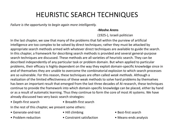
HEURISTIC SEARCH TECHNIQUES. Failure is the opportunity to begin again more intelligently. - Moshe Arens (1925-), Israeli politician

E N D
HEURISTIC SEARCH TECHNIQUES Failure is the opportunity to begin again more intelligently. -Moshe Arens (1925-), Israeli politician In the last chapter, we saw that many of the problems that fall within the purview of artificial intelligence are too complex to be solved by direct techniques; rather they must be attacked by appropriate search methods armed with whatever direct techniques are available to guide the search. In this chapter, a framework for describing search methods is provided and several general-purpose search techniques are discussed. These methods are all varieties of heuristic search. They can be described independently of any particular task or problem domain. But when applied to particular problems, their efficacy is highly dependent on the way they exploit domain-specific knowledge since in and of themselves they are unable to overcome the combinatorial explosion to which search processes are so vulnerable. For this reason, these techniques are often called weak methods. Although a realization of the limited effectiveness of these weak methods to solve hard problems by themselves has been an important result that emerged from the last three decades of AI research, these techniques continue to provide the framework into which domain-specific knowledge can be placed, either by hand or as a result of automatic learning. Thus they continue to form the core of most Al systems. We have already discussed two very basic search strategies: • Depth-first search • Breadth-first search In the rest of this chapter, we present some others: • Generate-and-test • Hill climbing • Best-first search • Problem reduction • Constraint satisfaction • Means-ends analysis
GENERATE-AND-TEST The generate-and-test strategy is the simplest of all the approaches we discuss. It consists of the following steps: Algorithm: Generate-and-Test 1. Generate a possible solution. For some problems, this means generating a particular point in the problem space. For others, it means generating a path from a start state. 2. Test to see if this is actually a solution by comparing the chosen point or the endpoint of the chosen path to the set of acceptable goal states. 3. If a solution has been found, quit. Otherwise, return to step 1. If the generation of possible solutions is done systematically, then this procedure will find a solution eventually, if one exists. Unfortunately, if the problem space is very large, "eventually" may be a very long time. The generate-and-test algorithm is a depth-first search procedure since complete solutions must be generated before they can be tested. In its most systematic form, it is simply an exhaustive search of the problem space. Generate-and-test can, of course, also operate by generating solutions randomly, but then there is no guarantee that a solution will ever be found. In this form, it is also known as the British Museum algorithm, a reference to a method for finding an object in the British Museum by wandering randomly. Between these two extremes lies a practical middle ground in which the search process proceeds systematically, but some paths are not considered because they seem unlikely to lead to a solution. This evaluation is performed by a heuristic function, as described in Section 2.2.2. The most straightforward way to implement systematic generate-and-test is as a depth-first search tree with backtracking. If some intermediate states are likely to appear often in the tree, however, it may be better to modify that procedure, as described above, to traverse a graph rather than a tree.
For simple problems, exhaustive generate-and-test is often a reasonable technique. For example, consider the puzzle that consists of four six-sided cubes, with each side of each cube painted one of four colors. A solution to the puzzle consists of an arrangement of the cubes in a row such that on all four sides of the row one block face of each color is showing. This problem can he solved by a person (who is a much slower processor for this sort of thing than even a very cheap computer) in several minutes by systematically and exhaustively trying all possibilities. It can be solved even more quickly using a heuristic generate-and-test procedure. A quick glance at the four blocks reveals that there are more, say, red faces than there are of other colors. Thus when placing a block with several red faces, it would be a good idea to use as few of them as possible as outside faces. As many of them as possible should be placed to abut the next block. Using this heuristic, many configurations need never be explored and a solution can be found quite quickly. Unfortunately, for problems much harder than this, even heuristic generate-and-test, all by itself, is not a very effective technique. But when combined with other techniques to restrict the space in which to search even further, the technique can be very effective. For example, one early example of a successful Al program is DENDRAL [Lindsay et aI., 1980], which infers the structure of organic compounds using mass spectrogram and nuclear magnetic resonance (NMR) data. It uses a strategy called plan-generate-test in which a planning process that uses constraint-satisfaction techniques (see Section 3.5) creates lists of recommended and contraindicated substructures. The generate-and- test procedure then uses those lists so that it can explore only a fairly limited set of structures. Constrained in this way, the generate-and-test procedure has proved highly effective. This combination of planning, using one problem-solving method (in this case, constraint satisfaction) with the use of the plan by another problem-solving method, generate-and-test, is an excellent example of the way techniques can be combined to overcome the limitations that each possesses individually.
A major weakness of planning is that it often produces somewhat inaccurate solutions since there is no feedback from the world. But by using it only to produce pieces of solutions that will then be exploited in the generate-and-test process, the lack of detailed accuracy becomes unimportant. And, at the same time, the combinatorial problems that arise in simple generate-and-test are avoided by judicious reference to the plans. HILL CLIMBING Hill climbing is a variant of generate-and-test in which feedback from the test procedure is used to help the generator decide which direction to move in the search space. In a pure generate-and-test procedure, the test function responds with only a yes or no. But if the test function is augmented with a heuristic function that provides an estimate of how close a given state is to a goal state, the generate procedure can exploit it as shown in the procedure below. This is particularly nice because often the computation of the heuristic function can be done at almost no cost at the same time that the test for a solution is being performed. Hill climbing is often used when a good heuristic function is available for evaluating states but when no other useful knowledge is available. For example, suppose you are in an unfamiliar city without a map and you want to get downtown. You simply aim for the tall buildings. The heuristic function is just distance between the current location and the location of the tall buildings and the desirable states are those in which this distance is minimized. Recall from Section 2.3.4 that one way to characterize problems is according to their answer to the question, "Is a good solution absolute or relative?” Absolute solutions exist whenever it is possible to recognize a goal state just by examining it. Getting downtown is an example of such a problem. For these problems, hill climbing can terminate whenever a goal state is reached. Only relative solutions exist, however, for maximization (or minimization) problems, such as the traveling salesman problem. In these problems, there is no a priori goal state. For problems of this sort, it makes sense to terminate hill climbing when there is no reasonable alternative state to move to.
Simple Hill Climbing The simplest way to implement hill climbing is as follows. Algorithm: Simple Hill Climbing I. Evaluate the initial state. If it is also a goal state, then return it and quit. Otherwise, continue with the initial state as the current state. 2. Loop until a solution is found or until there are no new operators left to be applied in the current state: (a) Select an operator that has not yet been applied to the current state and apply it to produce a new state. (b) Evaluate the new state. (i) If it is a goal state, then return it and quit. (ii) If it is not a goal state but it is better than the current state, then make it the current state. (iii) If it is not better than the current state, then continue in the loop. The key difference between this algorithm and the one we gave for generate-and-test is the use of an evaluation function as a way to inject task-specific knowledge into the control process. It is the use of such knowledge that makes this and the other methods discussed in the rest of this chapter heuristic search methods, and it is that same knowledge that gives these methods their power to solve some otherwise intractable problems. Notice that in this algorithm, we have asked the relatively vague question, “Is one state better than another” For the algorithm to work, a precise definition of better must be provided. In some cases, it means a higher value of the heuristic function. In others, it means a lower value. It does not matter which, as long as a particular hill-climbing program is consistent in its interpretation.
To see how hill climbing works, let's return to the puzzle of the four colored blocks. To solve the problem, we first need to define a heuristic function that describes how close a particular configuration is to being a solution. One such function is simply the sum of the number of different colors on each of the four sides. A solution to the puzzle will have a value of 16. Next we need to define a set of rules that describe ways of transforming one configuration into another. Actually, one rule will suffice. It says simply pick a block and rotate it 90 degrees in any direction. Having provided these definitions, the next step is to generate a starting configuration . This can either be done at random or with the aid of the heuristic function described in the last section. Now hill climbing can begin. We generate a new state by selecting a block and rotating it. If the resulting state is better, then we keep it. If not, we return to the previous slate and try a different interpretation. Steepest-Ascent Hill Climbing A useful variation on simple hill climbing considers all the moves from the current state and selects the best one as the next state. This method is called steepest-ascenthill climbing or gradient search. Notice that this contrast with the basic method in which the first state that is better than the current state is selected. The algorithm works as follows. Algorithm: Steepest-Ascent Hill Climbing 1. Evaluate the initial state. If it is also a goal state, then return it and quit. Otherwise, continue with the initial state as the current state. 2. Loop until a solution is found or until a complete iteration produces no change to current state: (a) Let SUCC be a state such that any possible successor of the current state will be better than SUCC. (b) For each operator that applies to the current state do: (i) Apply the operator and generate a new state. (ii) Evaluate the new state. If it is a goal state, then return it and quit. If not, compare it to SUCC. If it is better, then set SUCC to this state. If it is not better, leave SUCC alone.
(c) If the SUCC is better than current state, then set current state to SUCC. To apply steepest-ascent hill climbing to the colored blocks problem, we must consider all perturbations of the initial state and choose the best. For this problem, this is difficult since there are so many possible moves. There is a trade-off between the time required to select a move (usually longer for steepest-accent hill climbing) and the number of moves required to get to a solution (usually longer for basic hill climbing) that must be considered when deciding which method will work better for a particular problem. Both basic and steepest-ascent hill climbing may fail to find a solution. Either algorithm may terminate not by finding a goal state but by getting to a state from which no better states can be generated. This will happen if the program has reached either a local maximum, a plateau, or a ridge. A local maximum is a state that is better than all its neighbors but is not better than some other states farther away. At a local maximum, all moves appear to make things worse. Local maxima are particularly frustrating because they often occur almost within sight of a solution. In this case, they are called foothills. A plateau is a flat area of the search space in which a whole set of neighboring states have the same value. On a plateau, it is not possible to determine the best direction in which to move by making local comparisons. A ridge is a special kind of local maximum. It is an area of the search space that is higher than surrounding areas and that itself has a slope (which one would like to climb). But the orientation of the high region, compared to the set of available moves and the directions in which they move, makes it impossible to traverse a ridge by single moves.
There are some ways of dealing with these problems, although these methods are by no means guaranteed: Backtrack to some earlier node and try going in a different direction. This is particularly reasonable if at that node there was another direction that looked promising or almost as promising as the one that was chosen earlier. To implement this strategy, maintain a list of paths almost taken and go back to one of them if the path that was taken leads to a dead end. This is a fairly good way of dealing with local maxima. Make a big jump in some direction to try to get to a new section of the search space. This is a particularly good way of dealing with plateaus. If the only rules available describe single small steps, apply them several times in the same direction. Apply two or more rules before doing the test. This corresponds to moving in several directions at once. This is a particularly good strategy for dealing with ridges. Even with these first-aid measures, hill climbing is not always very effective. It is particularly unsuited to problems where the value of the heuristic function drops off suddenly as you move away from a solution. This is often the case whenever any sort of threshold effect is present. Hill climbing is a local method, by which we mean that it decides what to do next by looking only at the "immediate" consequences of its choice rather than by exhaustively exploring all the consequences. It shares with other local methods, such as the nearest neighbor heuristic described in Section 2.2.2, the advantage of being less combinatorially explosive than comparable global methods. But it also shares with other local methods a lack of a guarantee that it will be effective. Although it is true that the hill-climbing procedure itself looks only one move ahead and not any farther, that examination may in fact exploit an arbitrary amount of global information if that information is encoded in the heuristic function. Consider the blocks world problem shown in Fig. 3.1. Assume the same operators ( i.e., pick up one block and put it on the table; pick up one block and put it on another one) that were used in Section 2.3.1.
Suppose we use the following heuristic function: Local: Add one point for every block that is resting on the thing it is supposed to be resting on. Subtract one point for every block that is sitting on the wrong thing. Using this function, the goal state has a score of 8. The initial state has a score of 4 (since it gets one point added for blocks C, D, E, F, G, and H and one point subtracted for blocks A and B). There is only one move from the initial state, namely to move block A to the table. That produces a state with a score of 6 (since now A's position causes a point to be added rather than subtracted). The hill-climbing procedure will accept that move. From the new state, there are three possible moves, leading to the three states shown in Fig. 3.2. These states have the scores: (a) 4, (b) 4, and (c) 4. Hill climbing will halt because all these states have lower scores than the current state. The process has reached a local maximum that is not the global maximum. The problem is that by purely local examination of support structures, the current state appears to be better than any of its successors because more blocks rest on the correct objects. To solve this problem, it is necessary to disassemble a good local structure (the stack B through H) because it is in the wrong global context. We could blame hill climbing itself for this failure to look far enough ahead to find a solution. But we could also blame the heuristic function and try to modify it. Suppose we try the following heuristic function in place of the first one: Global: For each block that has the correct support structure (i.e. " the complete structure underneath it is exactly as it should be), add one point for every block in the support structure. For each block that has an incorrect support structure, subtract one point for every block in the existing support structure.
Using this function, the goal state has the score 28 (1 for B, 2 for C, etc,). The initial state has the score -- 28. Moving A to the table yields a state with a score of -- 21 since A no longer has seven wrong blocks under it. The three states that can be produced next now have the following scores: (a) -28, (b) -16, and (c) -15. This time, steepest-ascent hill climbing will choose move (c),which is the correct one. This new heuristic function captures the two key aspects of this problem: incorrect structures are bad and should be taken apart; and correct structures are good and should be built up. As a result, the same hill climbing procedure that failed with the earlier heuristic function now works perfectly. Unfortunately, it is not always possible to construct such a perfect heuristic function. For example, consider again the problem of driving downtown. The perfect heuristic function would need to have knowledge about one-way and dead-end streets, which, in the case of a strange city, is not always available. And even if perfect knowledge is, in principle, available, it may not be computationally tractable to use. As an extreme example, imagine a heuristic function that computes a value for a state by invoking its own problem-solving procedure to look ahead from the state it is given to find a solution. It then knows the exact cost of finding that solution and can return that cost as its value. A heuristic function that does this converts the local hill-climbing procedure into a global method by embedding a global method within it. But now the computational advantages of a local method have been lost. Thus it is still true that hill climbing can be very inefficient in a large, rough problem space. But it is often useful when combined with other methods that get it started in the right general neighborhood. Simulated Annealing Simulated annealing is a variation of hill climbing in which, at the beginning of the process, some downhill moves may be made. The idea is to do enough exploration of the whole space early on so that the final solution is relatively insensitive to the starting state. This should lower the chances of getting caught at a local maximum, a plateau, or a ridge.
In order to be compatible with standard usage in discussions of simulated annealing, we make two notational changes for the duration of this section . We use the term objective function in place of the term heuristic function. And we attempt to minimize rather than maximize the value of the objective function. Thus we actually describe a process of valley descending rather than hill climbing. Simulated annealing [Kirkpatrick et al., 1983] as a computational process is patterned after the physical process of annealing, in which physical substances such as metals are melted ( i.e., raised to high energy levels) and then gradually cooled until some solid state is reached. The goal of this process is to produce a minimal-energy final state. Thus this process is one of valley descending in which the objective function is the energy level. Physical substances usually move from higher energy configurations to lower ones, so the valley descending occurs naturally. But there is some probability that a transition to a higher energy state will occur. This is probability is given by the function p= e -∆E/kT where A £ is the positive change in the energy level T is the temperature, and k is Boltzmann's constant. Thus, in the physical valley descending that occurs during annealing, the probability of a large uphill move is lower than the probability of a small one. Also, the probability that an uphill move will be made decreases as the temperature decreases. Thus such moves are more likely during the beginning of the process when the temperature is high, and they become less likely at the end as the temperature becomes lower. One way to characterize this process is that downhill moves are allowed anytime. Large upward moves may occur early on, but as the process progresses, only relatively small upward moves are allowed until finally the process converges to a local minimum configuration. The rate at which the system is cooled is called the annealing schedule. Physical annealing processes are very sensitive to the annealing schedule. If cooling occurs too rapidly, stable regions of high energy will form.
In other words, a local but not global minimum is reached. If, however, a slower schedule is used, a uniform crystalline structure, which corresponds to a global minimum, is more likely to develop. But, if the schedule is too slow, time is wasted. At high temperatures, where essentially random motion is allowed, nothing useful happens. At low temperatures a lot of time may be wasted after the final structure has already been formed. The optimal annealing schedule for each particular annealing problem must usually be discovered empirically. These properties of physical annealing can be used to define an analogous process of simulated annealing, which can be used (although not always effectively) whenever simple hill climbing can be used. In this analogous process, ∆E is generalized so that it represents not specifically the change in energy but more generally, the change in the value of the objective function, whatever it is. The analogy for kTis slightly less straightforward. In the physical process, temperature is a well-defined notion, measured in standard units. The variable k describes the correspondence between the units of temperature and the units of energy. Since, in the analogous process, the units for both E and T are artificial, it makes sense to incorporate k into T, selecting values for T that produce desirable behavior on the part of the algorithm. Thus we use the revised probability formula P’= e -∆E/T But we still need to choose a schedule of values for T (which we still call temperature). We discuss this briefly below after we present the simulated annealing algorithm. The algorithm for simulated annealing is only slightly different from the simple hill-climbing procedure. The three differences are: • The annealing schedule must be maintained. • Moves to worse states may be accepted. • It is a good idea to maintain, in addition to the current state, the best state found so far. Then, if the final state is worse than that earlier state (because of bad luck in accepting moves to worse states), the earlier state is still available.
Algorithm: Simulated Annealing 1. Evaluate the initial state. If it is also a goal state, then return it and quit. Otherwise, continue with the initial state as the current state. 2. Initialize BEST-SO-FAR to the current state. 3. Initialize T according to the annealing schedule. 4. Loop until a solution is found or until there are no new operators left to be applied in the current state. (a) Select an operator that has not yet been applied to the current state and apply it to produce a new state. (b) Evaluate the new state. Compute ∆E = (value of current) - (value of new state) • If the new state is a goal state, then return it and quit. • If it is not a goal state but is better than the current state, then make it the current state. Also set BEST-SO-FAR to this new state. • If it is not better than the current state, then make it the current state with probability p' as defined above. This step is usually implemented by invoking a random number generator to produce a number in the range [0,1 ]. If that number is less than p', then the move is accepted. Otherwise, do nothing. (c) Revise T as necessary according to the annealing schedule. 5. Return BEST-SO-FAR as the answer.
To implement this revised algorithm, it is necessary to select an annealing schedule, which has three components. The first is the initial value to be used for temperature. The second is the criteria that will be used to decide when the temperature of the system should be reduced. The third is the amount by which the temperature will be reduced each time it is changed. There may also be a fourth component of the schedule, namely, when to quit. Simulated annealing is often used to solve problems in which the number of moves from a given state is very large (such as the number of permutations that can be made to a proposed traveling salesman route). For such problems, it may not make sense to try all possible moves. Instead, it may be useful to exploit some criterion involving the number of moves that have been tried since an improvement was found. Experiments that have been done with simulated annealing on a variety of problems suggest that the best way to select an annealing schedule is by trying several and observing the effect on both the quality of the solution that is found and the rate at which the process converges. To begin to get a feel for how to come up with a schedule, the first thing to notice is that as T approaches zero, the probability of accepting a move to a worse state goes to zero and simulated annealing becomes identical to simple hill climbing. The second thing to notice is that what really matters in computing the probability of accepting a move is the ratio ∆E/T. Thus it is important that values of T be scaled so that this ratio is meaningful. For example, T could be initialized to a value such that, for an average ∆E, p' would be 0.5. Chapter 18 returns to simulated annealing in the context of neural networks. BEST-FIRST SEARCH Until now, we have really only discussed two systematic control strategies, breadth-first search and depth-first search (of several varieties). In this section, we discuss a new method, best-first search, which is a way of combining the advantages of both depth-first and breadth-first search into a single method.
OR Graphs Depth-first search is good because it allows a solution to be found without all competing branches having to be expanded. Breadth-first search is good because it does not get trapped on dead-end paths. One way of combining the two is to follow a single path at a time, but switch paths whenever some competing path looks more promising than the current one does. At each step of the best-first search process, we select the most promising of the nodes we have generated so far. This is done by applying an appropriate heuristic function to each of them. We then expand the chosen node by using the rules to generate its successors. If one of them is a solution, we can quit. If not, all those new nodes are added to the set of nodes generated so far. Again the most promising node is selected and the process continues. Usually what happens is that a bit of depth-first searching occurs as the most promising branch is explored. But eventually, if a solution is not found, that branch will start to look less promising than one of the top-level branches that had been ignored. At that point, the now more promising, previously ignored branch will be explored. But the old branch is not forgotten. Its last node remains in the set of generated but unexpanded nodes. The search can return to it whenever all the others get bad enough that it is again the most promising path. Figure 3.3 shows the beginning of a best-first search procedure. Initially, there is only one node, so it will be expanded. Doing so generates three new nodes. The heuristic function, which, in this example, is an estimate of the cost of getting to a solution from a given node, is applied to each of these new nodes. Since node D is the most promising, it is expanded next, producing two successor nodes, E and F. But then the heuristic function is applied to them . Now another path, that going through node B, looks more promising, so it is pursued, generating nodes G and H. But again when these new nodes are evaluated they look less promising than another path, so attention is returned to the path through D to E. E is then expanded, yielding nodes I and J. At the next step, J will be expanded, since it is the most promising. This process can continue until a solution is found.
Notice that this procedure is very similar to the procedure for steepest-ascent hill climbing, with two exceptions. In hill climbing, one move is selected and all the others are rejected, never to be reconsidered. This produces the straightline behavior that is characteristic of hill climbing. In best-first search, one move is selected, but the others are kept around so that they can be revisited later if the selected path becomes less promising. Further, the best available state is selected in best-first search, even if that state has a value that is lower than the value of the state that was just explored. This contrasts with hill climbing, which will stop if there are no successor states with better values than the current state. Although the example shown above illustrates a best-first search of a tree, it is sometimes important to search a graph instead so that duplicate paths will not be pursued. An algorithm to do this will operate by searching a directed graph in which each node represents a point in the problem space. Each node will contain, in addition to a description or the problem state it represents, an indication of how promising it is, a parent link that points back to the best node from which it came, and a list of the nodes that were generated from it. The parent link will make it possible to recover the path to the goal once the goal is found. The list of successors will make it possible, if a better path is found to an already existing node, to propagate the improvement down to its successors. We will call a graph of this sort an OR graph, since each of its branches represents an alternative problem-solving path. To implement such a graph-search procedure, we will need to use two lists of nodes: • OPEN - nodes that have been generated and have had the heuristic function applied to them but which have not yet been examined (i.e., had their successors generated). OPEN is actually a priority queue in which the elements with the highest priority are those with the most promising value of the heuristic function. Standard techniques for manipulating priority queues can be used to manipulate the list. • CLOSED - nodes that have already been examined. We need to keep these nodes in memory if we want to search a graph rather than a tree, since whenever a new node is generated, we need to check whether it has been generated before.
We will also need a heuristic function that estimates the merits of each node we generate. This will enable the algorithm to search more promising paths first. Call this function f’ (to indicate that it is an approximation to a function/that gives the true evaluation of the node). For many applications, it is convenient to define this function as the sum of two components that we call g and h’. The function g is a measure of the cost of getting from the initial state to the current node. Note that g is not an estimate of anything; it is known to be the exact sum of the costs of applying each of the rules that were applied along the best path to the node. The function h' is an estimate of the additional cost of getting from the current node to a goal state. This is the place where knowledge about the problem domain is exploited. The combined function f', then, represents an estimate of the cost of getting from the initial state to a goal state along the path that generated the current node. If more than one path generated the node, then the algorithm will record the best one. Note that because g and h' must be added, it is important that h’ be a measure of the cost of getting from the node to a solution (i.e., good nodes get low values; bad nodes get high values) rather than a measure of the goodness of a node (i.e., good nodes get high values). But that is easy to arrange with judicious placement of minus signs. It is also Important that g be nonnegative. If this is not true, then paths that traverse cycles in the graph will appear to get better as they get longer. The actual operation of the algorithm is very simple. It proceeds in steps, expanding one node at each step, until it generates a node that corresponds to a goal state. At each step, it picks the most promising of the nodes that have so far been generated but not expanded. It generates the successors of the chosen node, applies the heuristic function to them , and adds them to the list of open nodes, after checking to see if any of them have been generated before. By doing this check, we can guarantee that each node only appears once in the graph, although many nodes may point to it as a successor. Then the next step begins. This process can be summarized as follows.
Algorithm: Best-First Search I. Start with OPEN containing just the initial state. 2. Until a goal is found or there are no nodes left on OPEN do: (a) Pick the best node on OPEN. (b) Generate its successors. (c) For each successor do: (i) If it has not been generated before, evaluate it, add it to OPEN, and record its parent. (ii) If it has been generated before, change the parent if this new path is better than the previous one. In that case, update the cost of getting to this node and to any successors that this node may already, have . The basic idea of this algorithm is simple. Unfortunately, it is rarely the case that graph traversal algorithms are simple to write correctly. And it is even rarer that it is simple to guarantee the correctness of such algorithms. In the section that follows, we describe this algorithm in more detail as an example of the design and analysis of a graph-search program. The A* Algorithm The best-first search algorithm that was just presented is a simplification of an algorithm called A*, which was first presented by Hart et al. [1968; 1972]. This algorithm uses the same f ‘, g, and h' functions, as well as the lists OPEN and CLOSED, that we have already described. Algorithm: A* l. Start with OPEN containing only the initial node. Set that node's g value to 0, its h' value to whatever it is, and its f' value to h' + 0, or h'. Set CLOSED to the empty list.
2. Until a goal node is found, repeat the following procedure: If there are no nodes on OPEN,report failure. Otherwise, pick the node on OPEN with the lowest f’ value. Call it BESTNODE. Remove it from OPEN. Place it on CLOSED. See if BESTNODE is a goal node. If so, exit and report a solution (either BESTNODE if all we want is the node or the path that has been created between the initial state and BESTNODE if we are interested in the path). Otherwise, generate the successors of BESTNODE but do not set BESTNODE to point to them yet. (First we need to see if any of them have already been generated.) For each such SUCCESSOR, do the following: (a) Set SUCCESSOR to point back to BESTNODE. These backwards links will make it possible to recover the path once a solution is found. (b) Compute g(SUCCESSOR) = g(BESTNODE) + the cost of getting from BESTNODE to SUCCESSOR. (c) See if SUCCESSOR is the same as any node on OPEN (i.e., It has already been generated but not processed). If so, call that node OLD. Since this node already exists in the graph, we can throw SUCCESSOR away and add OLD to the list of BESTNODE's successors. Now we must decide whether OLD's parent link should be reset to point to BESTNODE. It should be if the path we have just found to SUCCESSOR is cheaper than the current best path to OLD (since SUCCESSOR and OLD are really the same node). So see whether it is cheaper to getto OLD via its current parent or to SUCCESSOR via BESTNODE by comparing their g values. If OLD is cheaper (or just as cheap), then we need do nothing. If SUCCESSOR is cheaper, then reset OLD's parent link to point to BESTNODE, record the new cheaper path in g(OLD), and update f’(OLD).
(d) If SUCCESSOR was not on OPEN, see if it is on CLOSED. If so, call the node on CLOSED OLD and add OLD to the list of BESTNODE'ssuccessors. Check to see if the new path or the old path is better just as in step 2(c), and set the parent link-and g and f’ values appropriately. If we have just found a better path to OLD, we must propagate the improvement to OLD's successors. This is a bit tricky. OLD points to its successors. Each successor in turn points to its successors, and so forth, until each branch terminates with a node that either is still on OPEN or has no successors. So to propagate the new cost downward, do a depth-first traversal of the tree starting at OLD, changing each node's g value (and thus also its f' value), terminating each branch when you reach either a node with no successors or a node to which an equivalent or better path has already been found. This condition is easy to check for. Each node's parent link points back to its best known parent. As we propagate down to a node, see if its parent points to the node we are corning from. If so, continue the propagation. If not, then its g value already reflects the better path of which it is part. So the propagation may stop here. But it is possible that with the new value of g being propagated downward, the path we are following may become better than the path through the current parent. So compare the two. If the path through the current parent is still better, stop the propagation. If the path we are propagating through is now better, reset the parent and continue propagation. (c) If SUCCESSOR was not already on either OPEN or CLOSED, then put it on OPEN, and add it to the list of BESTNODE's successors. Compute f'(SUCCESSOR) = g(SUCCESSOR) + h'(SUCCESSOR).
Several interesting observations can be made about this algorithm. The first concerns the role of the g function. It lets us choose which node to expand next on the basis not only of how good the node itself looks (as measured by h'), but also on the basis of how good the path to the node was. By incorporating g into f’,we will not always choose as our next node to expand the node that appears to be closest to the goal. This is useful if we care about the path we find. If, on the other hand, we only care about getting to a solution somehow, we can define g always to be 0, thus always choosing the node that seems closest to a goal. If we want to find a path involving the fewest number of steps, then we set the cost of going from a node to its successor as a constant, usually 1. If, on the other hand, we want to find the cheapest path and some operators cost more than others, then we set the cost of going from one node to another to reflect those costs. Thus the A* algorithm can be used whether we are interested in finding a minimal-cost overall path or simply any path as quickly as possible. The second observation involves h’, the estimator of h, the distance of a node to the goal. If h' is a perfect estimator of h, then A* will converge immediately to the goal with no search. The better h’is, the closer we will get to that direct approach. If, on the other hand, the value of h' is always 0, the search will be controlled by g. If the valueof g is also 0, the search strategy will be random. If the value of g is always 1, the search will be breadth first. All nodes on one level will have lower g values, and thus lower f’ values than will all nodes on the next level. What if, on the other hand, h' is neither perfect nor 0? Can we say anything interesting about the behavior of the search? The answer is yes if we can guarantee that h' never overestimates h. In that case, the A* algorithm is guaranteed to find an optimal (as determined by g) path to a goal, if one exists. This can easily be seen from a few examples.
Consider the situation shown in Fig. 3.4. Assume that the cost of all arcs is 1. Initially, all nodes except A are on OPEN (although the Fig. shows the situation two steps later, after B and E have been expanded). For each node, f' is indicated as the sum of h' and g. In this example, node B has the lowest f’, 4, so it is expanded first. Suppose it has only one successor E, which also appears to be three moves away from a goal. Now f'(E) is 5, the same as f'(C). Suppose we resolve this in favor of the path we are currently following. Then we will expand E next. Suppose it too has a single successor F, also judged to be three moves from a goal. We are clearly using up moves and making no progress. But f’(F) = 6, which is greater than f'(C). So we will expand C next. Thus we see that by underestimating h'(B) we have wasted some effort. But eventually we discover that B was farther away than we thought and we go back and try another path. Now consider the situation shown in Fig. 3.5. Again we expand B on the first step. On the second step we again expand E. At the next step we expand F, and finally we generate G, for a solution path of length 4. But suppose there is a direct path from D to a solution, giving a path of length 2. We will never find it. By overestimating h'(D) we make D look so bad that we may find some other, worse solution without ever expanding D. In general, if h' might overestimate h, we cannot be guaranteed of finding the cheapest path solution unless we expand the entire graph until all paths are longer than the best solution . An interesting question is, "Of what practical significance is the theorem that if h’ never overestimates h then A* is admissible?" The answer is, "almost none," because, for most real problems, the only way to guarantee that h’ never overestimates h is to set it to zero. But then we are back to breadth-first search, which is admissible but not efficient. But there is a corollary to this theorem that is very useful. We can state it loosely as follows: Graceful Decay of Admissibility: If h' rarely overestimates h by more than δ,then the A* algorithm will rarely find a solution whose cost is more than δgreater than the cost of the optimal solution. The formalization and proof of this corollary will be left as an exercise.
The third observation we can make about the A* algorithm has to do with the relationship between trees and graphs. The algorithm was stated in its most general form as it applies to graphs. It can , of course, be simplified to apply to trees by not bothering to check whether a new node is already on OPEN or CLOSED. This makes it faster to generate nodes but may result In the same search being conducted many times if nodes are often duplicated. Under certain conditions, the A* algorithm can be shown to be optimal in that it generates the fewest nodes in the process of finding a solution to a problem. Under other conditions it is not optimal. For formal discussions of these conditions, see Gelperin [1977] and Martelli [1977].