Download
1 / 45
610 likes | 1.3k Views
Heuristic Search. Best First Search A* IDA* Beam Search Generate and Test Local Searches Hill Climbing Simple Hill Climbing Steepest Ascend Hill Climbing Stochastic Hill Climbing Simulated Annealing Local beam search Genetic Algorithms. State spaces. <S,P,I,G,W> - state space

E N D
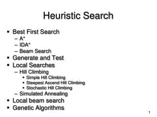
Heuristic Search Best First Search A* IDA* Beam Search Generate and Test Local Searches Hill Climbing Simple Hill Climbing Steepest Ascend Hill Climbing Stochastic Hill Climbing Simulated Annealing Local beam search Genetic Algorithms
State spaces <S,P,I,G,W> - state space S - set of states P= {(x,y)|x,yS} - set of production rules IS - initial state GS - set of goal states W: PR+ - weight function
Best first Search BestFirstSearch(state space =<S,P,I,G,W>,f) Open {<f(I),I>} Closed whileOpen do <fx,x> ExtractMin(Open) ifGoal(x, ) then return x Insert(x,Closed) for y Child(x ,)do if yClosed then Insert(<f(y),y>,Open) returnfail Open is implemented as a priority queue
Best First Search Example: The Eight-puzzle The task is to transform the initial puzzle • into the goal state • by shifting numbers up, down, left or right.
Best-First (Heuristic) Search 4 5 3 5 3 3 4 3 4 to the goal 3 to further unnecessary expansions
Best First Search - A* <S,P,I,G,W> - state space h*(x) - a minimum path weight from x to the goal state h(x) - heuristic estimate of h*(x) g(x) - a minimum path weight from I to x f(x) = g(x) + h(x)
Search strategies - A* A*Search(state space =<S,P,I,G,W>,h) Open {<h(I),0,I>} Closed whileOpen do <fx,gx,x> ExtractMin(Open) [minimum for fx] ifGoal(x, ) then return x Insert(<fx,gx,x>,Closed) for y Child(x ,)do gy = gx + W(x,y) fy = gy + h(y) if there is no <f,g,y>Closedwith ffythen Insert(< fy,gy,y>,Open) [replace existing <f,g,y>, if present] returnfail
Best-First Search (A*) 0+4 1+5 1+3 1+5 2+3 2+3 2+4 3+3 3+4 3+2 3+4 goal ! 5+0 4+1 5+2
Admissible search Definition An algorithm is admissible if it is guaranteed to return an optimal solution (with minimal possible path weight from the start state to a goal state) whenever a solution exists.
Admissibility What must be true about h for A* to find optimal path? 2 73 X Y h=1 h=100 1 1 h=0 h=0
Admissibility What must be true about h for A* to find optimal path? A* finds optimal path if h is admissible; h is admissible when it never overestimates. 2 73 X Y h=100 h=1 1 1 h=0 h=0
Admissibility What must be true about h for A* to find optimal path? A* finds optimal path if h is admissible; h is admissible when it never overestimates. In this example, h is not admissible. 2 73 X Y h=100 h=1 1 1 h=0 h=0 g(X)+h(X) = 102 g(Y)+h(Y) = 74 Optimal path is not found!
Admissibility of a Heuristic Function Definition A heuristic function h is said to be admissible if 0 h(n) h*(n) for all nS.
Optimality of A* (proof) Suppose some suboptimal goal G2has been generated and is in the fringe. Let n be an unexpanded node in the fringe such that n is on a shortest path to an optimal goal G. f(G2) = g(G2) since h(G2) = 0 f(G) = g(G) since h(G) = 0 g(G2) > g(G) since G2 is suboptimal f(G2) > f(G) from above
Optimality of A* (proof) Suppose some suboptimal goal G2has been generated and is in the fringe. Let n be an unexpanded node in the fringe such that n is on a shortest path to an optimal goal G. f(G2) > f(G) from above h(n) ≤ h*(n) since h is admissible g(n) + h(n) ≤ g(n) + h*(n) f(n) ≤ f(G), Hence f(G2) > f(n), and A* will never select G2 for expansion
Consistent heuristics A heuristic is consistent if for every node n, every successor n' of n generated by any action a, h(n) ≤ c(n,a,n') + h(n') If h is consistent, we have f(n') = g(n') + h(n') = g(n) + c(n,a,n') + h(n') ≥ g(n) + h(n) ≥ f(n) i.e., f(n) is non-decreasing along any path. Thus: If h(n) is consistent, A* using a graph search is optimal The first goal node selected for expansions is an optimal solution
Extreme Cases If we set h=0, then A* is Breadth First search; h=0 is admissible heuristic (when all costs are non-negative). If g=0 for all nodes, A* is similar to Steepest Ascend Hill Climbing If both g and h =0, it can be as dfs or bfs depending on the structure of Open
How to chose a heuristic? • Original problem PRelaxed problem P' A set of constraints removing one or more constraints P is complex P' becomes simpler • Use cost of a best solution path from n in P' as h(n) for P • Admissibility: h* h cost of best solution in P >= cost of best solution in P' Solution space of P Solution space of P'
How to chose a heuristic - 8-puzzle • Example: 8-puzzle • Constraints: to move from cell A to cell B cond1: there is a tile on A cond2: cell B is empty cond3: A and B are adjacent (horizontally or vertically) • Removing cond2: h2 (sum of Manhattan distances of all misplaced tiles) • Removing both cond2 and cond3: h1 (# of misplaced tiles) Here h2 h1
How to chose a heuristic - 8-puzzle h1(start) = 7 h2(start) = 18
Performance comparison Data are averaged over 100 instances of 8-puzzle, for varous solution lengths. Note: there are still better heuristics for the 8-puzzle.
Comparing heuristic functions Bad estimates of the remaining distance can cause extra work! Given two algorithms A1 and A2 with admissible heuristics h1and h2< h*(n), if h1(n) < h2(n) for all non-goal nodes n, then A1 expands at least as many nodes as A2 h2 is said to be more informed than h1 or, A2dominates A1
Weighted A* (WA*) fw(n) = (1–w)g(n) + w h(n) w = 0 - Breadth First w = 1/2 - A* w = 1 - Best First
IDA*: Iterative deepening A* To reduce the memory requirements at the expense of some additional computation time, combine uninformed iterative deepening search with A* Use an f-cost limit instead of a depth limit
Iterative Deepening A* In the first iteration, we determine a “f-cost limit”f’(n0) = g’(n0) + h’(n0) = h’(n0), where n0 is the start node. We expand nodes using the depth-first algorithm and backtrack whenever f’(n) for an expanded node n exceeds the cut-off value. If this search does not succeed, determine the lowest f’-value among the nodes that were visited but not expanded. Use this f’-value as the new limit value and do another depth-first search. Repeat this procedure until a goal node is found.
IDA* Algorithm - Top level function IDA*(problem) returns solution root :=Make-Node(Initial-State[problem]) f-limit:= f-Cost(root) loop do solution, f-limit := DFS-Contour(root, f-limit) if solution is not null,then return solution if f-limit = infinity, then return failure end
IDA* contour expansion function DFS-Countour(node,f-limit) returns solution sequence and new f-limit if f-Cost[node] > f-limit then return (null, f-Cost[node] ) if Goal-Test[problem](State[node]) then return (node,f-limit) for each node sin Successor(node) do solution, new-f := DFS-Contour(s, f-limit) if solution is not null,then return (solution, f-limit) next-f := Min(next-f, new-f); end return (null, next-f)
IDA*: Iteration 1, Limit = 4 0+4 1+5 1+3 2+3 2+3 2+4
IDA*: Iteration 2, Limit = 5 0+4 1+5 1+3 2+3 2+3 3+3 3+4 3+2 goal ! 5+0 4+1
Beam Search (with limit = 2) 0+4 1+5 1+3 1+5 2+3 2+3 2+4 3+3 3+4 3+4 3+2 goal ! 5+0 4+1 5+2
Generated and Test Algorithm Generate a (potential goal) state: Particular point in the problem space, or A path from a start state Test if it is a goal state Stop if positive go to step 1 otherwise Systematic or Heuristic? It depends on “Generate” 32
Local search algorithms In many problems, the path to the goal is irrelevant; the goal state itself is the solution State space = set of "complete" configurations Find configuration satisfying constraints, e.g., n-queens In such cases, we can use local search algorithms keep a single "current" state, try to improve it 33
Hill Climbing Simple Hill Climbing expand the current node evaluate its children one by one (using the heuristic evaluation function) choose the FIRST node with a better value Steepest Ascend Hill Climbing expand the current node Evaluate all its children (by the heuristic evaluation function) choose the BEST node with the best value 34
Hill-climbing Steepest Ascend 35
Hill Climbing Problems: local maxima problem plateau problem Ridge goal Ridge plateau goal 36
Drawbacks Ridge = sequence of local maxima difficult for greedy algorithms to navigate Plateaux = an area of the state space where the evaluation function is flat. 37
Hill-climbing example a) shows a state of h=17 and the h-value for each possible successor. b) A local minimum in the 8-queens state space (h=1). a) b) 38
Hill-climbing variations Stochastic hill-climbing Random selection among the uphill moves. The selection probability can vary with the steepness of the uphill move. First-choice hill-climbing Stochastic hill climbing by generating successors randomly until a better one is found. Random-restart hill-climbing A series of Hill Climbing searches from randomly generated initial states Simulated Annealing Escape local maxima by allowing some "bad" moves but gradually decrease their frequency 39
Simulated Annealing T = initial temperature x = initial guess v = Energy(x) Repeat while T > final temperature Repeat n times X’ Move(x) V’ = Energy(x’) If v’ < v then accept new x [ x x’ ] Else accept new x with probability exp(-(v’ – v)/T) T = 0.95T /* Annealing schedule*/ At high temperature, most moves accepted At low temperature, only moves that improve energy are accepted 40
Local beam search Keep track of k “current” states instead of one Initially: k random initial states Next: determine all successors of the k current states If any of successors is goal finished Else select k best from the successors and repeat. Major difference with k random-restart search Information is shared among k search threads. Can suffer from lack of diversity. Stochastic variant: choose k successors at proportionally to the state success. 41
Genetic algorithms • Variant of local beam search with sexual recombination. • A successor state is generated by combining two parent states • Start with k randomly generated states (population) • A state is represented as a string over a finite alphabet (often a string of 0s and 1s) • Evaluation function (fitness function). Higher values for better states. • Produce the next generation of states by selection, crossover, and mutation
Genetic algorithms • Fitness function: number of non-attacking pairs of queens (min = 0, max = 8 × 7/2 = 28) • 24/(24+23+20+11) = 31% • 23/(24+23+20+11) = 29% etc
Genetic algorithm function GENETIC_ALGORITHM( population, FITNESS-FN) return an individual input:population, a set of individuals FITNESS-FN, a function which determines the quality of the individual repeat new_population empty set loop for i from 1 to SIZE(population) do x RANDOM_SELECTION(population, FITNESS_FN) y RANDOM_SELECTION(population, FITNESS_FN) child REPRODUCE(x,y) if (small random probability) then child MUTATE(child ) add child to new_population population new_population until some individual is fit enough or enough time has elapsed return the best individual