Download
1 / 78
800 likes | 1.42k Views
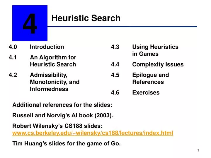
4 Heuristic Search 4.0 Introduction 4.1 An Algorithm for Heuristic Search 4.2 Admissibility, Monotonicity, and Informedness 4.3 Using Heuristics in Games 4.4 Complexity Issues 4.5 Epilogue and References 4.6 Exercises Additional references for the slides:

E N D
4 Heuristic Search 4.0 Introduction 4.1 An Algorithm for Heuristic Search 4.2 Admissibility, Monotonicity, and Informedness 4.3 Using Heuristics in Games 4.4 Complexity Issues 4.5 Epilogue and References 4.6 Exercises Additional references for the slides: Russell and Norvig’s AI book (2003). Robert Wilensky’s CS188 slides: www.cs.berkeley.edu/~wilensky/cs188/lectures/index.html Tim Huang’s slides for the game of Go.
Chapter Objectives • Learn the basics of heuristic search in a state space. • Learn the basic properties of heuristics: admissability, monotonicity, informedness. • Learn the basics of searching for two-person games: minimax algorithm and alpha-beta procedure. • The agent model: Has a problem, searches for a solution, has some “heuristics” to speed up the search.
Heuristic search of a hypothetical state space (Fig. 4.4) node The heuristic value of the node
Take the DFS algorithm • Function depth_first_search; • begin open := [Start]; closed := [ ]; while open [ ] do begin remove leftmost state from open, call it X; if X is a goal then return SUCCESS else begin generate children of X; put X on closed; discard remaining children of X if already on open or closed put remaining children on left end of open end end; return FAILend.
new Add the children to OPEN with respect to their heuristic value • Function best_first_search; • begin open := [Start]; closed := [ ]; while open [ ] do begin remove leftmost state from open, call it X; if X is a goal then return SUCCESS else begin generate children of X; assign each child their heuristic value; put X on closed; (discard remaining children of X if already on open or closed) put remaining children on opensort open by heuristic merit (best leftmost) end end; return FAILend. will be handled differently
Now handle those nodes already on OPEN or CLOSED • ... generate children of X; for each child of X do case the child is not on open or closed: begin assign the child a heuristic value; add the child to open end; the child is already on open: if the child was reached by a shorter path then give the state on open the shorter path the child is already on closed: if the child was reached by a shorter path then begin remove the child from closed; add the child to open end; end; put X on closed; re-order states on open by heuristic merit (best leftmost) end; ...
The full algorithm • Function best_first_search;begin open := [Start]; closed := [ ]; while open [ ] do begin remove leftmost state from open, call it X; if X is a goal then return SUCCESS else begin generate children of X; for each child of X do case the child is not on open or closed: begin assign the child a heuristic value; add the child to open end; the child is already on open: if the child was reached by a shorter path then give the state on open the shorter path the child is already on closed: if the child was reached by a shorter path then begin remove the child from closed; add the child to open end; end; put X on closed; re-order states on open by heuristic merit (best leftmost) end; return FAILend.
Heuristic search of a hypothetical state space with open and closed highlighted
What is in a “heuristic?” • f(n) = g(n) + h(n) The estimated cost of achieving the goal (from node n to the goal) The heuristic value of node n The actual cost of node n (from the root to n)
Algorithm A • Consider the evaluation function f(n) = g(n) + h(n) where n is any state encountered during the search g(n) is the cost of n from the start state h(n) is the heuristic estimate of the distance n to the goal • If this evaluation algorithm is used with the best_first_search algorithm of Section 4.1, the result is called algorithm A.
Algorithm A* • If the heuristic function used with algorithm A is admissible, the result is called algorithm A* (pronounced A-star). • A heuristic is admissible if it never overestimates the cost to the goal. • The A* algorithm always finds the optimal solution path whenever a path from the start to a goal state exists (the proof is omitted, optimality is a consequence of admissability).
Monotonicity • A heuristic function h is monotone if • 1. For all states ni and nJ, where nJ is a descendant of ni, • h(ni) - h(nJ) cost (ni, nJ), • where cost (ni, nJ) is the actual cost (in number of moves) of going from state ni tonJ. • 2. The heuristic evaluation of the goal state is zero, or h(Goal) = 0.
Informedness • For two A* heuristics h1 and h2, if h1 (n) h2 (n), for all states n in the search space, heuristic h2 is said to be moreinformed than h1.
Game playing • Games have always been an important application area for heuristic algorithms. The games that we will look at in this course will be two-person board games such as Tic-tac-toe, Chess, or Go.
First three levels of tic-tac-toe state space reduced by symmetry
A variant of the game nim • A number of tokens are placed on a table between the two opponents • A move consists of dividing a pile of tokens into two nonempty piles of different sizes • For example, 6 tokens can be divided into piles of 5 and 1 or 4 and 2, but not 3 and 3 • The first player who can no longer make a move loses the game • For a reasonable number of tokens, the state space can be exhaustively searched
Two people games • One of the earliest AI applications • Several programs that compete with the best human players: • Checkers: beat the human world champion • Chess: beat the human world champion (in 2002 & 2003) • Backgammon: at the level of the top handful of humans • Go: no competitive programs • Othello: good programs • Hex: good programs
Search techniques for 2-person games • The search tree is slightly different: It is a two-ply tree where levels alternate between players • Canonically, the first level is “us” or the player whom we want to win. • Each final position is assigned a payoff: • win (say, 1) • lose (say, -1) • draw (say, 0) • We would like to maximize the payoff for the first player, hence the names MAX & MINIMAX
The search algorithm • The root of the tree is the current board position, it is MAX’s turn to play • MAX generates the tree as much as it can, and picks the best move assuming that Min will also choose the moves for herself. • This is the Minimax algorithm which was invented by Von Neumann and Morgenstern in 1944, as part of game theory. • The same problem with other search trees: the tree grows very quickly, exhaustive search is usually impossible.
Special technique 1 • MAX generates the full search tree (up to the leaves or terminal nodes or final game positions) and chooses the best one: win or tie • To choose the best move, values are propogated upward from the leaves: • MAX chooses the maximum • MIN chooses the minimum • This assumes that the full tree is not prohibitively big • It also assumes that the final positions are easily identifiable • We can make these assumptions for now, so let’s look at an example
Two-ply minimax applied to X’s move near the end of the game (Nilsson, 1971)
Special technique 2 • Notice that the tree was not generated to full depth in the previous example • When time or space is tight, we can’t search exhaustively so we need to implement a cut-off point and simply not expand the tree below the nodes who are at the cut-off level. • But now the leaf nodes are not final positions but we still need to evaluate them: use heuristics • We can use a variant of the “most wins” heuristic
Calculation of the heuristic • E(n) = M(n) – O(n) where • M(n) is the total of My (MAX) possible winning lines • O(n) is the total of Opponent’s (MIN) possible winning lines • E(n) is the total evaluation for state n • Take another look at the previous example • Also look at the next two examples which use a cut-off level (a.k.a. search horizon) of 2 levels
Two-ply minimax applied to the opening move of tic-tac-toe (Nilsson, 1971)
Two-ply minimax and one of two possible second MAX moves (Nilsson, 1971)
Special technique 3 • Use alpha-beta pruning • Basic idea: if a portion of the tree is obviously good (bad) don’t explore further to see how terrific (awful) it is • Remember that the values are propagated upward. Highest value is selected at MAX’s level, lowest value is selected at MIN’s level • Call the values at MAX levels α values, and the values at MIN levels β values
The rules • Search can be stopped below any MIN node having a beta value less than or equal to the alpha value of any of its MAX ancestors • Search can be stopped below any MAX node having an alpha value greater than or equal to the beta value of any of its MIN node ancestors
Example with MAX α≥3 MAX MIN β=3 β≤2 MAX 4 5 2 3 (Some of) these still need to be looked at As soon as the node with value 2 is generated, we know that the beta value will be less than 3, we don’t need to generate these nodes (and the subtree below them)
Example with MIN β≤5 MIN MAX α=5 α≥6 MIN 4 5 6 3 (Some of) these still need to be looked at As soon as the node with value 6 is generated, we know that the alpha value will be larger than 6, we don’t need to generate these nodes (and the subtree below them)
Number of nodes generated as a function of branching factor B, and solution length L (Nilsson, 1980)
Informal plot of cost of searching and cost of computing heuristic evaluation against heuristic informedness (Nilsson, 1980)
Othello (a.k.a. reversi) • 8x8 board of cells • The tokens have two sides: one black, one white • One player is putting the white side and the other player is putting the black side • The game starts like this:
Othello • The game proceeds by each side putting a piece of his own color • The winner is the one who gets more pieces of his color at the end of the game • Below, white wins by 28
Othello • When a black token is put onto the board, and on the same horizontal, vertical, or diagonal line there is another black piece such that every piece between the two black tokens is white, then all the white pieces are flipped to black • Below there are 17 possible moves for white