Download

1 / 32
320 likes | 407 Views
Delve into decision trees' significant influences and variable relevance in complex functions for robust analysis. Learn about key influences and best practices in constructing decision trees. Uncover the importance of variables in shaping decision-making pathways for effective problem-solving.

E N D
Decision Trees and Influences Ryan O’Donnell - Microsoft Mike Saks - Rutgers Oded Schramm - Microsoft Rocco Servedio - Columbia
Printer troubleshooter Does anything print? Right size paper? Can print from Notepad? Network printer? Printer mis-setup? File too complicated? Solved Solved Driver OK? Driver OK? Solved Solved Call tech support
Decision tree complexity f : {Attr1} × {Attr2} × ∙∙∙ × {Attrn} → {−1,1}. What’s the “best” DT for f, and how to find it? Depth = worst case # of questions. Expected depth = avg. # of questions.
Building decision trees • Identify the most ‘influential’/‘decisive’/‘relevant’ variable. • Put it at the root. • Recursively build DTs for its children. Almost all real-world learning algs based on this – CART, C4.5, … Almost no theoretical (PAC-style) learning algs based on this – [Blum92, KM93, BBVKV97, PTF-folklore, OS04] – no; [EH89, SJ03] – sorta. Conj’d to be good for some problems (e.g., percolation [SS04]) but unprovable…
x2 x3 Boolean DTs f : {−1,1}n → {−1,1}. D(f) = min depth of a DT for f. 0 ≤ D(f) ≤ n. x1 x2 Maj3 −1 x3 1 −1 1 −1 1
Boolean DTs • {−1,1}n viewed as a probability space, with uniform probability distribution. • uniformly random path down a DT, plus a uniformly random setting of the unqueried variables, defines a uniformly random input • expected depth : δ(f).
Influences influence of coordinate j on f = the probability that xj is relevant for f Ij(f) = Pr[ f(x) ≠ f(x (⊕j)) ]. 0 ≤ Ij(f) ≤ 1.
Main question: If a function f has a “shallow” decision tree, does it have a variable with “significant” influence?
Main question: No. But for a silly reason: Suppose f is highly biased; say Pr[f = 1] = p ≪ 1. Then for any j, Ij(f) = Pr[f(x) = 1, f(x(j)) = −1] + Pr[f(x) = −1, f(x(j)) = 1] ≤ Pr[f(x) = 1] + Pr[f(x(j)) = 1] ≤ p + p = 2p.
Variance ⇒Influences are always at most 2 min{p,q}. Analytically nicer expression: Var[f]. • Var[f] = E[f2] – E[f]2 = 1 – (p – q)2 = 1 – (2p − 1)2 = 4p(1 – p) = 4pq. • 2 min{p,q} ≤ 4pq ≤ 4 min{p,q}. • It’s 1 for balanced functions. So Ij(f) ≤ Var[f], and it is fair to say Ij(f) is “significant” if it’s a significant fraction of Var[f].
Main question: If a function f has a “shallow” decision tree,does it have a variable with influence at leasta “significant” fraction of Var[f]?
Notation τ(d) = min max { Ij(f) / Var[f] }. f : D(f) ≤ d j
n Σ j = 1 Known lower bounds Suppose f : {−1,1}n → {−1,1}. • An elementary old inequality states Var[f] ≤ Ij(f). Thus f has a variable with influence at least Var[f]/n. • A deep inequality of [KKL88] shows there is always a coord. j such that Ij(f) ≥ Var[f] · Ω(log n / n). If D(f) = d then f really has at most 2d variables. Hence we get τ(d) ≥ 1/2d from the first, and τ(d) ≥ Ω(d/2d) from KKL.
x1 x3 x2 −1 1 1 −1 Our result τ(d) ≥ 1/d. This is tight: Then Var[SEL] = 1, d = 2, all three variables have infl. ½. (Form recursive version, SEL(SEL, SEL, SEL) etc., gives Var 1 fcn with d = 2h, all influences 2−h for any h.) “SEL”
n n n Σ Σ Σ j = 1 j = 1 j = 1 Our actual main theorem Given a decision tree f, let δj(f) = Pr[tree queries xj]. Then Var[f] ≤ δj(f)Ij(f). Cor: Fix the tree with smallest expected depth. Then δj(f) = E[depth of a path] =: δ(f) ≤ D(f). ⇒ Var[f] ≤ max Ij ·δj = max Ij · δ(f) ⇒ max Ij ≥ Var[f] / δ(f) ≥ Var[f] / D(f).
Proof Pick a random path in the tree. This gives some set of variables, P = (xJ1, … , xJT), along with an assignment to them, βP. Call the remaining set of variables P and pick a random assignment βP for them too. Let X be the (uniformly random string) given by combining these two assignments, (βP, βP). Also, define JT+1, … , Jn = ┴.
P P Proof Let β’P be an independent random asgn to vbls in P. Let Z = (β’P, βP). Note: Z is also uniformly random. JT+1= ··· = Jn = ┴ xJ1= –1 J1 J2 J3 JT xJ2= 1 X = (-1, 1, -1, …, 1, ) 1, -1, 1, -1 xJ3= -1 Z = ( , ) 1,-1, -1, …,-1 1, -1, 1, -1 xJT= 1 –1
Proof Finally, for t = 0…T, let Yt be the same string as X, except that Z’s assignments (β’P) for variables xJ1, … , xJt are swapped in. Note: Y0 = X, YT = Z. Y0 = X = (-1, 1, -1, …, 1, 1, -1, 1, -1 ) Y1= ( 1, 1, -1, …, 1, 1, -1, 1, -1 ) Y2 = ( 1,-1, -1, …, 1, 1, -1, 1, -1 ) · · · · YT = Z = ( 1,-1, -1, …,-1, 1, -1, 1, -1 ) Also define YT+1 = · · · = Yn = Z.
Σ Σ Σ Σ Σ Σ Σ t = 1..n t = 1..n t = 1..n t = 1..n j = 1..n t = 1..n j = 1..n Var[f] = E[f2] – E[f]2 = E[ f(X)f(X) ] – E[ f(X)f(Z) ] = E[ f(X)f(Y0) – f(X)f(Yn) ] = E[ f(X) (f(Yt−1) – f(Yt)) ] ≤ E[ |f(Yt−1) – f(Yt)| ] = 2 Pr[f(Yt−1) ≠ f(Yt)] = Pr[Jt = j] · 2 Pr[f(Yt−1) ≠ f(Yt) | Jt = j] = Pr[Jt = j] · 2 Pr[f(Yt−1) ≠ f(Yt) | Jt = j]
Σ Σ j = 1..n t = 1..n Proof … = Pr[Jt = j] · 2 Pr[f(Yt−1) ≠ f(Yt) | Jt = j] Utterly Crucial Observation: Conditioned on Jt = j, (Yt−1, Yt) are jointly distributed exactly as (W, W’), where W is uniformly random, and W’ is W with jth bit rerandomized.
P P JT+1= ··· = Jn = ┴ xJ1= –1 J1 J2 J3 JT xJ2= 1 Y0 = X = (-1, 1, -1, …, 1, 1, -1, 1, -1 ) Y1= ( 1, 1, -1, …, 1, 1, -1, 1, -1 ) Y2 = ( 1,-1, -1, …, 1, 1, -1, 1, -1 ) · · · · YT = Z = ( 1,-1, -1, …,-1, 1, -1, 1, -1 ) X = (-1, 1, -1, …, 1, ) 1, -1, 1, -1 xJ3= 1 Z = ( , ) 1,-1, -1, …,-1 1, -1, 1, -1 xJT= 1 –1
Σ Σ Σ Σ Σ Σ Σ Σ Σ j = 1..n j = 1..n j = 1..n j = 1..n t = 1..n t = 1..n j = 1..n t = 1..n t = 1..n Proof … = Pr[Jt = j] · 2 Pr[f(Yt−1) ≠ f(Yt) | Jt = j] = Pr[Jt = j] · 2 Pr[f(W) ≠ f(W’)] = Pr[Jt = j] · Ij(f) = Ij · Pr[Jt = j] = Ij δj.
Monotone graph properties v2 Consider graphs on v vertices; let n = (). “Nontrivial monotone graph property”: • “nontrivial property”: a (nonempty, nonfull) subset of all v-vertex graphs • “graph property”: closed under permutations of the vertices ( no edge is ‘distinguished’) • monotone: adding edges can only put you into the property, not take you out e.g.: Contains-A-Triangle, Connected, Has-Hamiltonian-Path, Non-Planar, Has-at-least-n/2-edges, …
Aanderaa-Karp-Rosenberg conj. Every nontrivial monotone graph propery has D(f) = n. [Rivest-Vuillemin-75]: ≥ v2/16. [Kleitman-Kwiatowski-80] ≥ v2/9. [Kahn-Saks-Sturtevant-84] ≥ n/2, = n, if v is a prime power. [Topology + group theory!] [Yao-88] = n in the bipartite case.
Randomized DTs • Have ‘coin flip’ nodes in the trees that cost nothing. • Or, probability distribution over deterministic DTs. Note: We want both 0-sided error and worst-case input. R(f) = min, over randomized DTs that compute f with 0-error, of max over inputs x, of expected # of queries. The expectation is only over the DT’s internal coins.
Maj3: D(Maj3) = 3. Pick two inputs at random, check if they’re the same. If not, check the 3rd. R(Maj3) ≤ 8/3. Let f = recursive-Maj3 [Maj3 (Maj3 , Maj3 , Maj3 ), etc…] For depth-h version (n = 3h), D(f) = 3h. R(f) ≤ (8/3)h. (Not best possible…!)
Randomized AKR / Yao conj. Yao conjectured in ’77 that every nontrivial monotone graph property f has R(f) ≥ Ω(v2). Lower bound Ω( · )Who v [Yao-77] v log 1/12 v [Yao-87] v5/4 [King-88] v4/3 [Hajnal-91] v4/3 log 1/3 v [Chakrabarti-Khot-01] min{ v/p, v2/log v } [Fried.-Kahn-Wigd.-02] v4/3 / p1/3 [us]
Outline • Extend main inequality to the p-biased case. (Then LHS is 1.) • Use Yao’s minmax principle: Show that under p-biased {−1,1}n, δ = Σ δj = avg # queries is large for any tree. • Main inequality: max influence is small ⇒ δ is large. • Graph property all vbls have the same influence. • Hence: sum of influences is small ⇒ δ is large. • [OS04]: f monotone ⇒ sum of influences ≤ √δ. • Hence: sum of influences is large ⇒ δ is large. • So either way, δ is large.
Generalizing the inequality n Σ Var[f] ≤ δj(f)Ij(f). Generalizations (which basically require no proof change): • holds for randomized DTs • holds for randomized “subcube partitions” • holds for functions on any product probability space f : Ω1× ∙∙∙ ×Ωn → {−1,1} (with notion of “influence” suitably generalized) • holds for real-valued functions with (necessary) loss of a factor, at most √δ j = 1
Closing thought It’s funny that our bound gets stuck roughly at the same level as Hajnal / Chakrabarti-Khot, n2/3 = v4/3. Note that n2/3 [I believe] cannot be improved by more than a log factor merely for monotone transitive functions, due to [BSW04]. Thus to get better than v4/3 for monotone graph properties, you must use the fact that it’s a graph property. Chakrabarti-Khot does definitely use the fact that it’s a graph property (all sorts of graph packing lemmas). Or do they? Since they get stuck at essentially v4/3, I wonder if there’s any chance their result doesn’t truly need the fact that it’s a graph property…