Download
1 / 47
480 likes | 485 Views
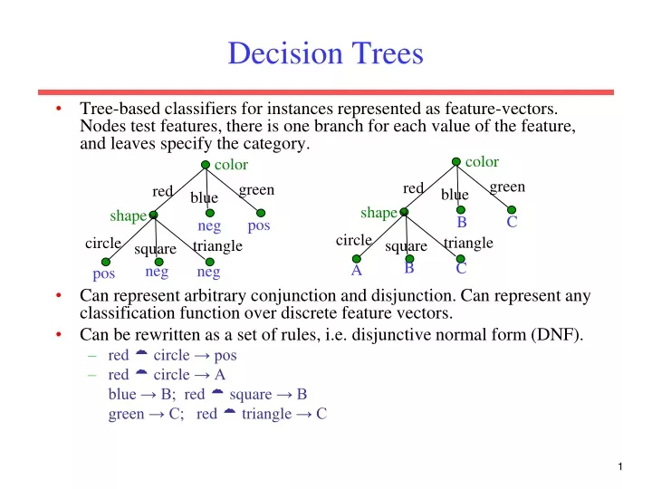
color. color. green. green. red. red. blue. blue. shape. shape. pos. C. neg. B. circle. circle. triangle. triangle. square. square. B. neg. C. neg. pos. A. Decision Trees.

E N D
color color green green red red blue blue shape shape pos C neg B circle circle triangle triangle square square B neg C neg pos A Decision Trees • Tree-based classifiers for instances represented as feature-vectors. Nodes test features, there is one branch for each value of the feature, and leaves specify the category. • Can represent arbitrary conjunction and disjunction. Can represent any classification function over discrete feature vectors. • Can be rewritten as a set of rules, i.e. disjunctive normal form (DNF). • red circle → pos • red circle → A blue → B; red square → B green → C; red triangle → C
Properties of Decision Tree Learning • Continuous (real-valued) features can be handled by allowing nodes to split a real valued feature into two ranges based on a threshold (e.g. length < 3 and length 3) • Classification trees have discrete class labels at the leaves, regression trees allow real-valued outputs at the leaves. • Algorithms for finding consistent trees are efficient for processing large amounts of training data for data mining tasks. • Methods developed for handling noisy training data (both class and feature noise). • Methods developed for handling missing feature values.
color green red blue Top-Down Decision Tree Induction • Recursively build a tree top-down by divide and conquer. <big, red, circle>: + <small, red, circle>: + <small, red, square>: <big, blue, circle>: <big, red, circle>: + <small, red, circle>: + <small, red, square>:
color green red blue shape circle triangle square Top-Down Decision Tree Induction • Recursively build a tree top-down by divide and conquer. <big, red, circle>: + <small, red, circle>: + <small, red, square>: <big, blue, circle>: <big, red, circle>: + <small, red, circle>: + <small, red, square>: neg neg <big, blue, circle>: pos neg pos <big, red, circle>: + <small, red, circle>: + <small, red, square>:
Decision Tree Induction Pseudocode DTree(examples, features) returns a tree If all examples are in one category, return a leaf node with that category label. Else if the set of features is empty, return a leaf node with the category label that is the most common in examples. Else pick a feature F and create a node R for it For each possible value vi of F: Let examplesi be the subset of examples that have value vi for F Add an out-going edge E to node R labeled with the value vi. If examplesi is empty then attach a leaf node to edge E labeled with the category that is the most common in examples. else call DTree(examplesi , features– {F}) and attach the resulting tree as the subtree under edge E. Return the subtree rooted at R.
Picking a Good Split Feature • Goal is to have the resulting tree be as small as possible, per Occam’s razor. • Finding a minimal decision tree (nodes, leaves, or depth) is an NP-hard optimization problem. • Top-down divide-and-conquer method does a greedy search for a simple tree but does not guarantee to find the smallest. • General lesson in ML: “Greed is good.” • Want to pick a feature that creates subsets of examples that are relatively “pure” in a single class so they are “closer” to being leaf nodes. • There are a variety of heuristics for picking a good test, a popular one is based on information gain that originated with the ID3 system of Quinlan (1979).
Entropy • Entropy (disorder, impurity) of a set of examples, S, relative to a binary classification is: where p1 is the fraction of positive examples in S and p0 is the fraction of negatives. • If all examples are in one category, entropy is zero (we define 0log(0)=0) • If examples are equally mixed (p1=p0=0.5), entropy is a maximum of 1. • Entropy can be viewed as the number of bits required on average to encode the class of an example in S where data compression (e.g. Huffman coding) is used to give shorter codes to more likely cases. • For multi-class problems with c categories, entropy generalizes to:
2+, 2 : E=1 shape 2+, 2 : E=1 size 2+, 2 : E=1 color big small 1+,1 1+,1 E=1 E=1 red blue 2+,1 0+,1 E=0.918 E=0 circle square 2+,1 0+,1 E=0.918 E=0 Gain=1(0.51 + 0.51) = 0 Gain=1(0.750.918 + 0.250) = 0.311 Gain=1(0.750.918 + 0.250) = 0.311 Information Gain • The information gain of a feature F is the expected reduction in entropy resulting from splitting on this feature. where Sv is the subset of S having value v for feature F. • Entropy of each resulting subset weighted by its relative size. • Example: • <big, red, circle>: + <small, red, circle>: + • <small, red, square>: <big, blue, circle>:
Hypothesis Space Search • Performs batchlearning that processes all training instances at once rather than incremental learning that updates a hypothesis after each example. • Performs hill-climbing (greedy search) that may only find a locally-optimal solution. Guaranteed to find a tree consistent with any conflict-free training set (i.e. identical feature vectors always assigned the same class), but not necessarily the simplest tree. • Finds a single discrete hypothesis, so there is no way to provide confidences or create useful queries.
Hypothesis Space Search by ID3 • Hypothesis space is complete • Target function surely in there … • Output a single hypothesis (which one?) • Do not have the ability to determine how many alternative decision trees are consistent with the training data • Can not pose new instance queries to resolve among competing hypothesis • No back tracking • Local minima • Statistically-based search choices • Robust to noisy data • Inductive bias: approx “prefer shortest tree”
Inductive Bias in ID3 • Note H is the power set of instances X • Unbiased? • Not really • Preference for short trees, and for those with high information gain attributes near the root • It chooses the first acceptable tree it encounters in its simple-to-complex, hill-climbing search • Selects in favor of shorter trees • Selects trees that place the attributes with highest information gain closest to the root • Bias is a preference for some hypotheses, rather than a restriction of hypothesis space H • Occam’s razor: prefer the shortest hypothesis that fits the data
Occam’s Razor • Why prefer short hypotheses? • Argument in favor: • Fewer short hypotheses than long ones • A short hypothesis that fits data unlikely to be coincidence • A long hypothesis that fits data might be coincidence • Argument opposed • There are many ways to define small sets of hypotheses • e.g. all trees with a prime number of nodes that use attributes beginning with “Z” • What’s so special about small sets based on size of hypothesis • The size of a hypothesis is determined by the particular representation used internally
Bias in Decision-Tree Induction • Information-gain gives a bias for trees with minimal depth. • Implements a search (preference) bias instead of a language (restriction) bias.
History of Decision-Tree Research • Hunt and colleagues use exhaustive search decision-tree methods (CLS) to model human concept learning in the 1960’s. • In the late 70’s, Quinlan developed ID3 with the information gain heuristic to learn expert systems from examples. • Simulataneously, Breiman and Friedman and colleagues develop CART (Classification and Regression Trees), similar to ID3. • In the 1980’s a variety of improvements are introduced to handle noise, continuous features, missing features, and improved splitting criteria. Various expert-system development tools results. • Quinlan’s updated decision-tree package (C4.5) released in 1993. • Weka includes Java version of C4.5 called J48.
Weka J48 Trace 1 data> java weka.classifiers.trees.J48 -t figure.arff -T figure.arff -U -M 1 Options: -U -M 1 J48 unpruned tree ------------------ color = blue: negative (1.0) color = red | shape = circle: positive (2.0) | shape = square: negative (1.0) | shape = triangle: positive (0.0) color = green: positive (0.0) Number of Leaves : 5 Size of the tree : 7 Time taken to build model: 0.03 seconds Time taken to test model on training data: 0 seconds
on training data on test data Overfitting • Learning a tree that classifies the training data perfectly may not lead to the tree with the best generalization to unseen data. • There may be noise in the training data that the tree is erroneously fitting. • The algorithm may be making poor decisions towards the leaves of the tree that are based on very little data and may not reflect reliable trends. • A hypothesis, h, is said to overfit the training data is there exists another hypothesis which, h´, such that h has less error than h´ on the training data but greater error on independent test data. accuracy hypothesis complexity
Overfitting Noise in Decision Trees • Category or feature noise can easily cause overfitting. • Add noisy instance <medium, blue, circle>: pos (but really neg) color red blue green shape neg neg circle triangle square pos neg pos
big med small neg pos neg Overfitting Noise in Decision Trees • Category or feature noise can easily cause overfitting. • Add noisy instance <medium, blue, circle>: pos (but really neg) color red blue green <big, blue, circle>: <medium, blue, circle>: + shape neg circle triangle square pos neg pos • Noise can also cause different instances of the same feature vector to have different classes. Impossible to fit this data and must label leaf with the majority class. • <big, red, circle>: neg (but really pos) • Conflicting examples can also arise if the features are incomplete and inadequate to determine the class or if the target concept is non-deterministic.
Notes on Overfitting • Overfitting results in decision trees that are more complex than necessary • Training error no longer provides a good estimate of how well the tree will perform on previously unseen records • Need new ways for estimating errors
Overfitting Prevention (Pruning) Methods • Two basic approaches for decision trees • Prepruning: Stop growing tree as some point during top-down construction when there is no longer sufficient data to make reliable decisions. • Postpruning: Grow the full tree, then remove subtrees that do not have sufficient evidence. • Label leaf resulting from pruning with the majority class of the remaining data, or a class probability distribution. • Method for determining which subtrees to prune: • Cross-validation: Reserve some training data as a hold-out set (validation set, tuning set) to evaluate utility of subtrees. • Statistical test: Use a statistical test on the training data to determine if any observed regularity can be dismissed as likely due to random chance. • Minimum description length (MDL): Determine if the additional complexity of the hypothesis is less complex than just explicitly remembering any exceptions resulting from pruning.
How to Address Overfitting • Pre-Pruning (Early Stopping Rule) • Stop the algorithm before it becomes a fully-grown tree • Typical stopping conditions for a node: • Stop if all instances belong to the same class • Stop if all the attribute values are the same • More restrictive conditions: • Stop if number of instances is less than some user-specified threshold • Stop if class distribution of instances are independent of the available features (e.g., using 2 test) • Stop if expanding the current node does not improve impurity measures (e.g., Gini or information gain).
How to Address Overfitting… • Post-pruning • Grow decision tree to its entirety • Trim the nodes of the decision tree in a bottom-up fashion • If generalization error improves after trimming, replace sub-tree by a leaf node. • Class label of leaf node is determined from majority class of instances in the sub-tree • Can use MDL for post-pruning
Estimating Generalization Errors • Re-substitution errors: error on training data e(t) • Generalization errors: e’(t) • Methods for estimating generalization errors: • Optimistic approach: e’(t) = e(t) • Pessimistic approach: • For each leaf node: e’(t) = (e(t)+0.5) • Total errors: e’(T) = e(T) + N 0.5 (N: number of leaf nodes) • For a tree with 30 leaf nodes and 10 errors on training (out of 1000 instances): Training error = 10/1000 = 1% Generalization error = (10 + 300.5)/1000 = 2.5% • Reduced error pruning (REP): • uses validation data set to estimate generalization error
Reduced Error Pruning • A post-pruning, cross-validation approach. Partition training data in “grow” and “validation” sets. Build a complete tree from the “grow” data. Until accuracy on validation set decreases do: For each non-leaf node, n, in the tree do: Temporarily prune the subtree below n and replace it with a leaf labeled with the current majority class at that node. Measure and record the accuracy of the pruned tree on the validation set. Permanently prune the node that results in the greatest increase in accuracy on the validation set.
Issues with Reduced Error Pruning • The problem with this approach is that it potentially “wastes” training data on the validation set. • Severity of this problem depends where we are on the learning curve: test accuracy number of training examples
Example of Post-Pruning Training Error (Before splitting) = 10/30 Pessimistic error = (10 + 0.5)/30 = 10.5/30 Training Error (After splitting) = 9/30 Pessimistic error (After splitting) = (9 + 4 0.5)/30 = 11/30 PRUNE!
C0: 11 C1: 3 C0: 14 C1: 3 C0: 2 C1: 4 C0: 2 C1: 2 Examples of Post-pruning Case 1: • Optimistic error? • Pessimistic error? • Reduced error pruning? Don’t prune for both cases Don’t prune case 1, prune case 2 Case 2: Depends on validation set
Occam’s Razor • Given two models of similar generalization errors, one should prefer the simpler model over the more complex model • For complex models, there is a greater chance that it was fitted accidentally by errors in data • Therefore, one should include model complexity when evaluating a model
Minimum Description Length (MDL) • Cost(Model,Data) = Cost(Data|Model) + Cost(Model) • Cost is the number of bits needed for encoding. • Search for the least costly model. • Cost(Data|Model) encodes the misclassification errors. • Cost(Model) uses node encoding (number of children) plus splitting condition encoding.
Rule Post-Pruning • Convert tree to equivalent set of rules • Prune each rule independently of others • Sort final rules into desired sequence for use Perhaps most frequently used method (e.g., C4.5)
Why convert decision tree to rules before pruning? • Converting to rules allow distinguishing among the different contexts in which a decision node is used • Pruning decision about attribute test can be made differently for different paths • Converting to rules removes the distinction between attribute tests that occur near the root of the tree and those occur near the leaves. • Converting to rules improves readability
Additional Decision Tree Issues • Better splitting criteria • Information gain prefers features with many values. • Continuous features • Predicting a real-valued function (regression trees) • Missing feature values • Features with costs • Misclassification costs • Incremental learning • ID4 • ID5 • Mining large databases that do not fit in main memory
Handling Missing Attribute Values • Missing values affect decision tree construction in three different ways: • Affects how impurity measures are computed • Affects how to distribute instance with missing value to child nodes • Affects how a test instance with missing value is classified
Computing Impurity Measure Before Splitting:Entropy(Parent) = -0.3 log(0.3)-(0.7)log(0.7) = 0.8813 Split on Refund: Entropy(Refund=Yes) = 0 Entropy(Refund=No) = -(2/6)log(2/6) – (4/6)log(4/6) = 0.9183 Entropy(Children) = 0.3 (0) + 0.6 (0.9183) = 0.551 Gain = 0.9 (0.8813 – 0.551) = 0.3303 Missing value
Distribute Instances Refund Yes No Probability that Refund=Yes is 3/9 Probability that Refund=No is 6/9 Assign record to the left child with weight = 3/9 and to the right child with weight = 6/9 Refund Yes No
Classify Instances New record: Refund Yes No NO MarSt Single, Divorced Married Probability that Marital Status = Married is 3.67/6.67 Probability that Marital Status ={Single,Divorced} is 3/6.67 TaxInc NO < 80K > 80K YES NO