Download

1 / 31
310 likes | 542 Views
Ch 2 and 9.1 Relationships Between 2 Variables. More than one variable can be measured on each individual. Examples: Gender and Height Size and Cost Eye color and Major We want to look at the relationship among these variables. Is there an association between these two variables?

E N D
Ch 2 and 9.1Relationships Between 2 Variables • More than one variable can be measured on each individual. • Examples: • Gender and Height • Size and Cost • Eye color and Major • We want to look at the relationship among these variables. • Is there an association between these two variables? • Two variables measured on the same individuals are associated if some values tend to occur more often with some values of the second variable than with other values of that variable.
Relationships Between 2 Variables • If we expect one variable to influence another, we call it the ___________ variable. • Explains or influences changes in the response variable • The variable that is influenced is called the ____________ variable. • Measures an outcome of a study • In each of the following examples, identify the explanatory and response variables • Gender and blood pressure • Class attendance and course grade • Number of beers and BAC
Relationships Between 2 Variables • We may be interested in relationships of different types of variables. • Categorical and Numeric • Categorical and Categorical • Numeric and Numeric
Relationships between Categorical and Numeric Variables • We are interested in comparing the numerical variable across each of the levels of the categorical variable. • Examples: • Compare high speeds for 4 different car brands • Compare sucrose levels for 5 different types of fruit • Compare GPR for 20 different majors
Relationships between Categorical and Numeric Variables • Graphical Comparison • Example: Sucrose levels of fruits (fictitious data)
Relationships between Categorical and Numeric Variables • Numerical Comparison • We could also look at summary statistics for each group.
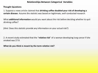
Ch 9.1Relationships Between Two Categorical Variables • Depending on the situation, one of the variables is the explanatory variable and the other is the response variable. • In this case, we look at the percentages of one variable for each level of the other variable. • Examples: • Gender and Soda Preference • Country of Origin and Marital Status • Smoking Habits and Socioeconomic Status
Two-Way Tables • Two-way tables come about when we are interested in the relationship between two categorical variables. • One of the variables is the _____________. • The other is the _______________. • The combination of a row variable and a column variable is a ______________.
Column variable Cells Row Totals Column Totals Row variable Overall Total Two-Way Tables • Example:
Relationships between two categorical variables • Example: Gender and Highest Degree Obtained • Joint Distribution: How likely are you to have a bachelor’s degree and be a male? _____________ • Marginal Distribution: What is the least likely highest degree obtained? _____________ • Conditional Distribution: If you are a female, how likely are you to have obtained a graduate degree? ______________
Relationships between two categorical variables Shows the percentages for the joint, marginal, and conditional distributions.
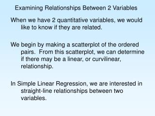
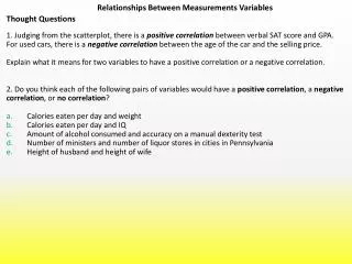
Ch 2 Relationships Between 2 Numeric Variables • Depending on the situation, one of the variables is the explanatory variable and the other is the response variable. • There is not always an explanatory-response relationship. • Examples: • Height and Weight • Income and Age • SAT scores on math exam and on verbal exam • Amount of time spent studying for an exam and exam score
Relationships between 2 numeric variables • Scatterplots • Look for overall pattern and any striking deviations from that pattern. • Look for outliers, values falling outside the overall pattern of the relationship • You can describe the overall pattern of a scatterplot by the form, direction, and strength of the relationship. • Form: Linear or clusters • Direction • Two variables are _____________________ when above-average values of one tend to accompany above-average values of the other and likewise below-average values also tend to occur together. • Two variables are _____________________ when above-average values of one variable accompany below-average values of the other variable, and vice-versa. • Strength-how close the points lie to a line
___________Association Relationships between 2 numeric variables • Example: • Response: MPG • Explanatory: Weight Response Variable (y-axis) Explanatory Variable (x-axis)
__________ Association Relationships between 2 numeric variables • Relationships between two numeric variables • Example • Vehicle Weight • Horsepower
Relationships between 2 numeric variables • ___________ or r: measures the direction and strength of the linear relationship between two numeric variables • General Properties • It must be between -1 and 1, or (-1≤r≤ 1). • If r is negative, the relationship is negative. • If r = –1, there is a perfect negative linear relationship (extreme case). • If r is positive, the relationship is positive. • If r = 1, there is a perfect positive linear relationship (extreme case). • If r is 0, there is no linear relationship. • r measures the strength of the linear relationship. • If explanatory and response are switched, r remains the same. • r has no units of measurement associated with it • Scale changes do not affect r
Relationships between 2 numeric variables • Examples of extreme cases r = 1 r = 0 r = -1
Relationships between 2 numeric variables • Match the correlation with to the scatterplot r = 0.04 r =0.43 r = -0.84 r = 0.76 r = 0.21
Relationships between 2 numeric variables It is possible for there to be a strong relationship between two variables and still have r ≈ 0. EX.
Relationships between 2 numeric variables • Important notes: • Association does not imply causation • Correlation does not imply causation • Slope is not correlation • A scale change does not change the correlation. • Correlation doesn’t measure the strength of a non-linear relationship:
Regression Line • A regression line is a straight line that describes how a response variable y changes as an explanatory variable x changes. • A regression line summarizes the relationship between two variables, but only in a specific setting: when one of the variables helps explain or predict the other. • We often use a regression line to predict the value of y for a given value of x. • Regression, unlike correlation, requires that we have an explanatory variable and a response variable
Regression Line • Fitting a line to data means drawing a line that comes as close as possible to the points. • Extrapolation-the use of a regression line for prediction far outside the range of values of the explanatory variable x that you used to obtain the line. • Such predictions are often not accurate.
Least-Squares Regression Line • The least-squares regression line of y on xis the line that makes the sum of squares of the vertical distances of the data points from the line as small as possible. • These vertical distances are called the residuals, or the error in prediction, because they measure how far the point is from the line: where y is the point and is the predicted point.
Least-Squares Regression Line • The equation of the least-squares regression line of y on xis
Least-Squares Regression Line • The expression for slope, b1, says that along the regression line, a change of one standard deviation in x corresponds to a change of r standard deviations in y. • The slope, b1, is the amount by which y changes when x increases by one unit. • The intercept, b0, is the value of y when • The least-squares regression line ALWAYS passes through the point
r2 in Regression • The square of the correlation, r2, is the fraction of the variation in the values of y that is explained by the least-squares regression of y on x. • Use r2 as a measure of how successfully the regression explains the response. • Interpret r2 as the “percent of variation explained” • For Simple Linear Regression, r2is simply the square of the correlation coefficient.
Relationships between 2 numeric variables • Example How much of the variation is explained by the least squares line of y on x? ______ What is the correlation coefficient? ______ Horsepower = -10.78 + 0.04*weight (Equation of the line.) __________: y-value or response (horsepower) when line crosses the y-axis. _______: increase in response for a unit increase in explanatory variable. So if weight increases by one pound, horsepower increases by 0.04 units (on average).
Relationships between 2 variables Lurking Variable: A variable that is not among the explanatory or response variables in a study and yet may influence the interpretation of relationships among those variables. Simpson’s Paradox: An association or comparison that holds for all of several groups can reverse direction when the data are combined to form a single group. This reversal is called Simpson’s Paradox. This can happen when a lurking variable is present. Please see Examples 9.9 and 9.10 in the text.
Outliers and Influential Observations in Regression • An outlier is an observation that lies outside the overall pattern of the other observations. • An observation is influential for a statistical calculation if removing it would markedly change the result of the calculation. • Points that are outliers in the x direction of a scatterplot are often influential for the least-squares regression line.
Outliers and Influential Observations in Regression Child 18 is an outlier in the x direction. Because of its extreme position on the age scale, this point has a strong influence on the position of the regression line. r2 is also affected by the influential observation. With Child 18, r2 = 41%, but without Child 18, r2 = 11%. The apparent strength of the association was largely due to a single influential observation. The dashed line was calculated leaving out Child 18. The solid line is with Child 18.