Download
1 / 38
380 likes | 508 Views
Previous lecture: Fundamentals of radio astronomy. Flux, brightness temperature... Antennae, surface accuracy, antenna temperature... Signal & noise. Detecting a weak signal. Some general considerations. Blazar observing techniques. Word of warning:

E N D
Previous lecture:Fundamentals of radio astronomy • Flux, brightness temperature... • Antennae, surface accuracy, antenna temperature... • Signal & noise. • Detecting a weak signal. • Some general considerations.
Blazar observing techniques Word of warning: It is possible that your friendly support staff has no experience whatsoever from blazar observations! Special considerations: continuum sources of unknown fluxes (variable!) faint sources sources that may not be suitable for pointing (faint) absolute calibration needs to be accurate exercise special caution if looking for IDV!!!!!!
Receivers, problem areas • Noise from the recei ver, gain fluctuations etc.: large factor compared to the astronomical signal. • Signal-to-noise ratio radio astronomical measurements arealso measuring ”noise”! • Signal << background. • Power levels are low (P ca. 10-15 - 10-20 W). • Noise also from ground, atmosphere, etc.
We need: • Good stability. • Good sensitivity. • Good measurement techniques (elimination of background etc.).
Background noise • Man-made noise • Receiver itself, cables & other components, other radio signals (GSM!), etc. • Noise from the nature: • Atmosphere, CMB, black body radiation from ground etc., Solar radiation, thunderstorms ...
Receivers • Heterodyne receivers • Defining technologies: HEMT, Schottky, SIS. • Bolometers. • Bolometer arrays. • Especially in the receiver technology considerable differences btw. microwave / millimetre / submm!
Heterodyne receiver= Superheterodyne or super receiver, ”superhet” ~ • Uses a local oscillator at a freqeuency that is different from the incoming signal, to obtain an itermediate frequency that isprocessed using conventional microwave technology. • Different technologies at different frequency ranges,HEMT amplifiers vs. SIS mixers,currently the limiting freqeuency ca. 100 GHz. telescope sideband filter Dicke-switch mixer pre-amplifier IF amplifier detector comparison load localoscillator
Preamplifier • At lower freqeuencies, f <~ 120 GHz(note: upper freq-limit changing with new technologies!) • At higher frequencies not in use (too noisy, or nonexistent). • Common abbreviations: • LNA = Low Noise Amplifier. • HEMT = High Electron Mobility Transistor.
Sideband filtering • Not desirable/useful in continuum observations! • Normally two sidebands, upper sideband (USB) and lower sideband (LSB), get through the mixer. • Used for sideband rejection, before the mixer,to filter one of the sidebands --> single sideband, SSB. • For continuum observations, wide bandwidth is desired and both sidebands carry information: double sideband, DSB. • If sideband rejection is normally in use, check if you canget rid of it for continuum work!
Mixer • The signal gets converted (”mixed”) to a lower frequency. • Amplifying high radio frequencies (mm/submm) is difficult, amplifiying low-freq signals is easy. • (Especially earlier) no preamplifiers for high f exist(ed), only amplifying after mixing possible. • Signal frequency fs, local oscillator frequency fLO lower intermediate frequency fIF = | fs – fLO| fIF much lower, much easier to handle (= amplify).
Mixer technologies • Schottky diode • Older technology, easy to build. • Typically for lower frequencies & ambient temperatures. • SIS junction mixer (Superconductor-Insulator Supercond.) • Requires cooling, more challenging to build. • For frequencies > 100 GHz (at lower freqs no direct benefit & requires more maintenance),widely in use at mm/submm telescopes especially for spectral line work. • Useful for detecting faint signals, ie. when high sensitivity is needed. • In practise often problems with stability! • Bolometers much preferred for continuum work!
Local oscillator • Typically a semiconductor oscillator that can be phaselocked to an exact frequency. • Most common: Gunn oscillator.Difficult to make for n > 120 GHz: multipliers.Gunn oscillator itself not very stable: phase locking to a more stable oscillator.Phase lock loop (PLL) keeps the Gunn LO stable (n & phase). • Output signal: intermediate frequency, IF. • Stability required especially for spectral line observations and VLBI. At high frequencies stability may be a problem.
Dicke-switching • Gain fluctuations from mixers. • Varying background noise. • Observed signal e.g. 1/10000 of the overall system noise. • Amplifications by a factor of ca. 1012 may be desired. comparison measurement by Dicke-switching (R.H. Dicke 1946).
... Dicke switching • Swithching rate e.g. 5 – 100 Hz. • Reference source: noise diode; attenuator; signal from the blank sky(e.g., two-feedhorn method in Metsähovi). • Two beam-method for beam switching: two feedhorns or one beam + chopper wheel.
Millimetre-domain:special considerations • Components are small. • Tolerances are small. • Components are often expensive. • Circuit losses larger than in the microwave region. • Amplifier technology still in development. • Less power. • Atmospheric attenuation is large. • Millimetre domain technology: • Quasioptics (Mirrors, lenses; diffraction must be taken into account!) • Cooling is necesssary.
Quasioptics • In the (sub)mm domain the interface from the telescope to the detector. • Mirrors, lenses, grids are small geometrical optics can not be used (diffraction) Gaussian optics = quasioptics: optimizes the feeds of the receiver to the antenna beam pattern. • Can include a polarizer plate.
Cryostat • SIS requires very low temperatures. • Helium cooling. • Cooled parts of the receiver in vacuum container, dewar. • Dewar enclosed in a radiation shield. • Radiation shield cooled by a closed-cycle refrigerator.
Bolometer • A total power detector. • High sensitivity from a cooled device. • Wide bandwidth. • Relatively easy to construct & operate. Classical semiconductor bolometers Superconducting TES devices Silicon pop-up detectors (PUDs)
... Bolometer • Classical Germanium bolometer. • The temperature rise causes a change in the resistance of the bolometer and consequently in the voltage across it. V is amplified and measured.
Bolometer characteristics • Noise Equivalent Power, NEP= The power absorbed that prduces a S/N of unity at the bolometer output.NEP2 = NEP2(detector) + NEP2(background) • Thermal time constant t= a measure of the response time of the bolometer to incoming radiation= C/G • Compromise btw response time and NEP! • In practise, with wide bandwith the bolometer performance can degrade due to power loading from the background “background” = loading + photon noise.
Bolometer arrays • Until mid-1990’s bolometers were mainly single-channel devices. • Main advantage: mapping of extended sources, i.e. not directly applicable for blazar studies. • Can eliminate the need for separate pointing observations (depending on the obs. configuration).
Bolometer arrays currently in use • SCUBA @JCMT • 450 / 850 mm, 91/37 pixels, 300/65 mJy/sqrt(Hz). • MAMBO-2 @IRAM • 350 mm, 384 pixels, 500 mJy/sqrt(Hz). • Many hundreds or even thousands of pixels. • Silicon-micro machining, thin-film deposition and hybridization techniques. • Integrated SQUID multiplexers in the same plane as the detector chip. • E.g., SCUBA-2: 10000 pixels, for JCMT.SPIRE for HERSCHEL: 200-700 microns, 3 arrays of 43, 88 and 139 pixels. Future:
Observing techniques: beam switching • Source size, line/continuum, etc: --> Observing method (Position switching, Frequency swithching, Load Switching) • Continuum observations of point sources: beam switching. • Single beam switching: The source is in the signal beam, the sky is observed in the reference beam. • Dual beam switching: Alternates the source/sky in the signal and reference beams. • Dual beam switching produces good results when sky noise is the problem = most of the time • Note: ON/ON, ON/OFF terminology not fully standard! • Technology: dual horn setup or chopper; nodding secondary; telescope movement.
... beam switching, things to remember • Relatively large overheads: do not use too short integration times per beam. • Data reduction: make sure to know whether your intensities are to be divided by 2 or not!
Dual beam switching A II B I A B • 2 feedhorns / beams, A & B • Dicke-swithcing: measures signal A – signal B (integrated in e.g. 1 s chunks). I A: background (b) B: background + source (b + s) II A: background + source (b + s) B: background (b) (s + b)B - bA D = 2S bB – (s + b)A Not the same background! Eliminates e.g. effects of a radome very well!
Point source observations... • 1-point observation, problems:One must rely on the pointing pattern & offsets required earlier. • Drift scans:The moving source ”drifts” over the beam.Gaussian fit Smax. • 5-point observation:For relatively bright sources!Default ”center” point + 4 other positions.2-dimensional Gaussian fit: amplitude + offsets.
Pointing • Radio telescope pointing can never be quite perfect:telescope size, gravitaional deformation, heating(more exotic problems: pedestial tilts, earth quakes, ...) • Pointing pattern. • Pointing checks. • 5-point (9-point) measurement: offsetsamplitude correction (2-dimensional gaussian fit).
Focusing • Antenna deformation may be caused by gravitaional or wind forces, or by differential thermal expansion. illumination pattern is controlled by changingthe position/shape of the secondary mirror Very important in the submm region!
Calibration • From the observed DV or DT into Sobserved. • Load calibration (noise diode, chopper wheel). • Opacity (tau) measurements (skydips). • Flux calibration. • (Pointing check: sometimes called ”pointing calibration”).
... calibration • cm-frequencies: noise diode injection for receiver calibration: Gain fluctuations (temperature, electronics, mechanical stress). • mm-frequencies: absorbing blakcbody load (blocks the sky emission, corrects for atmospheric attenuation), can be done frequently ”corrected antenna temperature” TA* • Skydips: • Take up observing time. • Assume homogeneous, plane-parallel atmosphere. • Corrections usually done at data reduction stage. • Primary flux calibrator: a bright source with a known, constant flux. • Secondary calibrator:a bright ”relatively well-known, relatively constant flux”.
... calibration • Microwave domain: primary: DR21, Jupiter, Mars;secondary: e.g., 3C274, 3C84.(”Baars scale”). • Submillimetre domain: primary: Mars, Uranus;secondary: planetary nebulae, giant stars, ultracompact HII... • Consult the support staff for advise on the observatory calibration procedures + suitable calibrators & their flux information! • Always make sure to make frequent flux calibrator observations!!!
... calibration • Tau measurements / skydips: • Measure the noise temperature of the sky at various elevations. • Effect on the flux calibration: exp(tau/sin(el)).
Telescope performance, sky noise • Performance is represented by the Noise Equivalent Flux Density (NEFD). • Depends very much on the weather and varies with sky transmission. • Often the fundamental sensitivity limit is set by the ”sky noise”. • Sky noise spatial and temporal variations in the emissivity of the atmosphere. • Sky noise can degrade the NEFD by more than an order of magnitude. • Chopped beams travel through slightly different atmospheric paths Use narrow beam switching! Still some residual. • With a bolometer array one can try to remove large-scale effects to high order.
From an observation into a data point • Observing strategy: • Is focusing needed? • Is load calibration needed? • Is skydip needed? • Choose target source. Bright enough for a pointing source?No: check pointing or use reliable offsets in the same direction. • Observe source, keep an eye on S/N if possible;if not, make a quick-look analysis to check if integration time was optimal. • Observe calibrator source.Avoid unnesessary slewing, avoid blind pointing, make sure to keep an eye on the weather changes, observe primary and secondary calibrators often enough!
... From an observation into a data point • Data reduction: • Enough flux calibration data? • Enough tau information? • Was the weather OK all through your run? • Bolometer array data: reduce the image following local instructions. • Single channel bolometer or heterodyne data: obtain the average result of the various ON/ON pairs with their cumulative error. • Make tau corrections + any other general corrections. • Obtain flux conversion factors from the calibrators.Are they consistent??? • Use the FCFs for your own sources. • Error estimates from rms values + deviations in FCFs.
Bolometer data reduction • E.g. SCUBA photometry:Flatfielding; Extinction correction; Despiking; Examine individual bolometer quality & change if needed;Sky removal; Average or parabola fit over the 9-point map;Catenation of individual measurements
How to write a good proposal or: ” OK you think you’ve got a good science case...but THEY don’t know it! • Why this telescope? • Why this/these observing band(s)? • Read the manuals: observing manuals, data reduction,show them that you understand it all. • Any specific constraints? Sun, gain/elevation,weather, pointing, ... • Work out the realistic integration times including realistic overheads, explain them all. • If using heterodyne receiver, pay attention to:tuningsidebandsbackenddata reduction
Observational radio astronomy • N. Bartel et al. 1987, ApJ 323. 507:“No data were taken at station D during the period 0830 to 1630 GST due to the presence of a red racer snake (Coluber constrictor) draped across the high-tension wires (33,000 V) serving the station. However, even though this snake, or rather a three-foot section of its remains, was caught in the act of causing an arc between the transmission lines, we do not consider it responsible for the loss of data. Rather we blame the incompetence of a red tailed hawk (Buteo borealis) who had apparently built a defective nest that fell off the top of the nearby transmission tower, casting her nestlings to the ground, along with their entire food reserve consisting of a pack rat, a kangaroo rat, and several snakes, with the exception of the above-mentioned snake who had a somewhat higher destiny. No comparable loss of data occurred at the other antenna sites.”