Download
1 / 93
960 likes | 1.16k Views
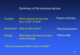
Plasma chemistry. Plasma propulsion. Plasma light. Summary of the previous lecture. Particles: Which species do we have how “much” of each. Momentum: How do they move? . Energy: What about the thermal motion internal energy . What do we want/need to know in detail?. Particles.

E N D
Plasma chemistry Plasma propulsion Plasma light Summary of the previous lecture Particles: Which species do we have how “much” of each Momentum: How do they move? Energy: What about the thermal motion internal energy What do we want/need to know in detail?
Particles Plasma Particles Energy Energy Momentum Momentum Particles: Plasma Chemistry Energy: Plasma Light Momentum: Plasma Propulsion
Hybride Quasi Free Flight mean free paths large mfp > L Sampling and tracking Transport Modes Fluid mean free paths small mfp << L There are many conditions for which some plasma components behave “fluid-like” whereas others are more “particle-like” Hybride models have large application fields
Source Discretizing a Fluid: Control Volumes Plasma Particles Particles Energy Energy Momentum Momentum For any transportable quantity Transport via boundaries
How many species? Examples of transportables Densities Momenta in three directions Mean energy (temperature) Depends on Equilibrium departure As we will see: In many fluid/hybrid cases Energy: 2T: {e} and {h} Momentum: for the bulk Navier Stokes for the species: Drift Diffusion Species: the transport sensitive
Mean properties Nodal Points Transport at boundaries = Source, t + = S Steady State Transient General structure: = u -D Convection Diffusion Nodal Point communicating via Boundaries Transport Fluxes: Linking CV (or NP’s) -
Other Example: Poisson: .E = /o = S = u -D E = - V Simularities Thus: The Fluid Eqns: Balance of Particles Momentum Energy The Momenta of the Boltzmann Transport Eqn. Thus no “convection” Can all be Treated as -equations
The Variety D S Temperature Heat cond Heat gen Momentum Viscosity Force Density Diffusion Creation Molecules atoms ions/electrons etc.
T Continuum t + = S Tin Rod Tout x 0 + T = 0 Take k = Cst MathNumerics: a FlavorSourceless-Diffusion T = Cst T = - kT -T /k =T
Continuum Tin Rod Tout Discretized Intuition; T = Cst T2 = (T1 + T3)/2 1 2 3 4 Tin -2T1 + T2= 0 T1 - 2T2 + T3 = 0 T2 - 2T3 + T4 = 0 T3 - 2T4 + Tout = 0 2T2 = T1 + T3 Discretized
In matrix: M T = b A Sparce Matrix Many zeros Matrix Representation 1 2 3 4 -Tin 0 0 -Tout T1 T2 T3 T4 1 2 3 4 - 2 1 1 -2 1 1 -2 1 1 -2 =
Sourceless-Diffusion in two dimensions 1 1 – 4 1 1 N W P E S T5 = (T2 + T4 +T6 + T8 ) /4 Provided k = Cst !! In general:
If k Cst Convection Diffusion More general S-less Diffusion/Convection
= u -D = S = -D If no “convection” Poisson Laplace - D = S S 0 S=0 - D = 0 - D = S Laplace and Poisson
Ohms’ law Space charge Ener balance Ion balance .E = /o .j = 0 j = E . E = 0 E = -V -.Dn = Ion - Rec -.kT = S -. V = /o -.V = 0 Examples Simularities !!
N Each V the Average of the two adjacent V d A Capacitor space-charge zero -. V = /o = 0 0 +V Basically a 1-D problem
+V 0 N Each V the Average of the two adjacent V d A resistor: Ohms law -.V = 0 1-D problem Provided is Cst
Source of ions Example ions: n+u+ = P+ - n+D+ Recombination Ordering the Sources = S S = P - L L ~ D Source combination Production and Loss Large local - value in general leads to large Loss
t = Nt Concept disturbed Bilateral Relations A proper channel N f N b Equilibrium Condition: t/b << 1 or t b << 1 The escape per balance time must be small
N D t = Nt N D Mixed Channel P - nD = n u The larger D The less important transport for The more local chemistry determined Note D is more general than bin dBR: collective chemistry
Cells are needed To organize the field contributions Ingredients for non-fluid codes The more equilibrium is abandoned the more info we need Tracking the particles: Integrating Eqn of Motion F = ma Interaction by chance: Monte Carlo Field contructions: a) positions giving charge density E b) motion giving current density B
Fluid versus particles (swarms) Particle codes Directly binary interacting individual particles Bookkeeping Position/velocity Each indivual part Particle in cell interaction via self-made field Sampling Distribution Over r and v Hybride particles in a fluid environment Distribution function Known in shape Continuum
A quasi free flight example Radiative Transfer • Ray-Trace Discretization spectrum. • Network of lines (rays) • Compute I (W/(m2 .sr.Hz) along the lines • Start outside the plasma with I() = 0. • Entering plasma I() grows afterwards absorption. • dI()/ds = j- k()I()
General Procedure ?? Fluid Swarm Collection {h} {i} {e} {} {h} {i} {es} {ef} {} E {h} {i} {es}{ef} {} E {h} {i} {es}{ef} {} E {h} {i} {es}{ef} {} Pressure
The BTE: basic form The BTE deals with fi(r,v,t) defined such that fi(r,v,t)d3rd3v the number of particles of kind “i” in a volume d3r of the configuration space centered around r with a velocity in the velocity space element d3v around v. Examples e A, A+, A*, A**, etc, N, N2, etc. NH, H2 Note that “i” may refer to an atom in a ground state the same atom in an excited state An ion or molecule, etc. etc. The BTE states that: tfi + .fiv + v.fia = (tfi)CR
Source S tn accumulation . nv and/or Efflux Simularities of the Boltzmann Transport equation tn + . nv = S Leads to
Generalization to 6-D phase space Normal space tn + . nv = S Accumulation Transport Source tfi + .fiv = (tfi)CR Phase space The Boltzmann Transport Eqn
The BTE: general form Use the divergence in the 6 dim space (r x v). tfi + .fiv = (tfi)CR BTE: Shorthand notation This is a equation in space Representing tfi + .fiv + v.fia = (tfi)CR
I Multiply BTE for “i”with a function g(v) and integrate over v. For each species: specific balances of mass; charge; current; momentum; energy Higher structures units: Elements; Bulk: mass; charge; current; momentum; energy II From Micro to Macro ordering using BTE Fluid approach: assume shape of f is known Procedure
g(v) tni + .niui = Spart, i Particle 1 0-mom Mass mi tni mi + .ni miui = Smass,i Momentum BTE miv tfi + .fiv = (tfi/dt)CR qi Charge tni qi+ .ni qiui = Scharge,i, 1-mom tni i+ .ni iui = Senergy,i =1/2miv2 2-mom Energy tni miui+ .ni miuiui = Smom, i, The momenta of the BTE: Specific balances Note: is in configaration space solely u is systematic velocity in configuration space Smom contains p and .: This approach is questionable
tni + .niui = Spart, i Particle 1 Mass mi tni mi + .ni miui = Smass,i qi Charge tni qi+ .ni qiui = Scharge,i The zero order momenta Note that Smass,i = mi Spart,i Scharge,i = qi Spart,i
ti ui+ . iiuiui = -pi+ .i+ i g +ni qiE+ niqiuiB + Fij, or Drift/Diffusion equation: 0 = -p +ni qiE+ Fij, Simplifications for specific mom balance ui is omnipresent: simplifications of the origen: mom bal tni miui + .ni miuiui = Smom, i, In many cases: ti ui+. iiuiui , niqiuiB and i g negligible p, ni qiEand Fij, dominant
0 = -pi + ni qiE+ Fij, F = Ffric + Fthermo Fijfric = (pipj/pDij) (uj– ui) Case one dominant species with udom= u p = pdom pi = ni kTi ni (ui –u)= - (Di/ kTi ) pi + (ni qiDi/ kTi ) E, Drift Diffusion continued Mostly: Ffric >> Fthermo Fijfric = -(pipdom /pDij) (ui - u) Fijfric = -(pi/Di) (ui- u) Fijfric = -(kTi /Di) {ni (ui- u)}
Thus ni (ui– u )= - (Di/ kTi ) pi +(ni i) E or ni (ui– u )= - Dini +(ni ) E With i = qiDi/kTi If T 0 Einstein relation Drift - Diffusion II Normally: ni (ui– u )= - (Di/ kTi ) pi + (ni qiDi/ kTi ) E,
E = -1 (j + i qi ipi) or E = Ej + Eamb ne eqe qe e >> qii Ambipolar Diffussion ni(ui– u )= - (Di/ kTi ) pi +(ni i) E with i = qiDi/kTi mobility and = i nii qi conductivity j = i niqi (ui– u )= - i ipi +E In most cases the current density jis closely related to the external control parameter I; and E the result Eamb = -1i qi ipi Eamb = {kTe /qe}pe/pe
For the ions ni(ui– u )= - (Di/ kTi ) pi + niDi{Te/Ti } {qi /qe}pe/pe, For the electrons neqeue = j Beware of the signs!!
Since Smass = m Spart Reaction Conservatives I : mass AB A+ B mAB = mA + mB Reactions Each creation of couple A and B associated with disappearence AB SAB = - SA = -SB Thus SAB mAB + mASA + mBSB =0 More general all mi Spart, i = 0 or all Smass, i = 0
Since Scharge = q S Reaction Conservative II: charge AB A+ + B- qAB = qA + qB Reactions SAB = - SA = -SB Each creation of couple A and B associated with destruction AB Thus qAB SAB + qASA+ qBSB=0 More general all qi Si = 0 or all Scharge,i = 0
all Smass,i = 0 tni mi + .ni miui = Smass,i all all all Scharge,i = 0 The Composition Bulk in Mass tm + . mu = 0 gives with m = all nimi and u nimiui /m barycentric or bulk velocity Bulk in Charge tq + . j = 0 t ni qi + .ni qiui = Scharge,i With j = ni q1ui Current density
Reaction Conservatives III: Nuclei In general: species can be composed e.g. NH3 is composed out of one N nucleus and three H We say R of N in NH3 = 1 or RN(NH3) = 1 and R of H in NH3 = 3 or RH(NH3) = 3 or Ri = 3 with “i” = NH3 and “” = H Now consider NH3 N + 3H RH(NH3) Spart(NH3) = RH(N) Spart(N) + RH(H) 3 Spart(H) In general: all RH(i) Spart,i = 0
all RHj Spart, j= 0 tni RHi + .niRHiuj = Smass,i all Elemental transport of H t {H} + . {H} = 0 gives With ni RHi = {H} and {H} = niRHiuj In steady state: . {H} = 0
In general t {X} + . {X} = 0 The change in time of the number density of nuclei of type X Equals minus the efflux of these nuclei; The efflux {X}of X is the weigthed sum: {X} = RXij j=niuj Number of X nuclei in j Efflux of “j”
Removing 1 H atom Equivalent: removing 3 H atoms Removing 1 H3 molecule {H} = 3 H3 In general: {H} = RHij
all mj Spart,j= 0 all RHj Spart,j = 0 tni mi + .ni miuj = Smass,i tni RXi + .niRXiuj = Smass,i all all all all qj Spart,j = 0 Simularities Total mass transport tm + . mu = 0 Total charge transport tq + . j = 0 tni qj + .ni qiuj = Scharge,i Total X-nuclei transport t {X} + . {X} = 0
=0 = 0 Charge neutrality Action = -Reaction The momentum balance on higher structure levels The elements: simple addition of the DD equation. The bulk: i { ti ui+ . iuiui = -pi+ .i+ i g +ni qiE+ ni qiuiB+ Fij } Navier Stokes tu+ . uu = -p+ .+ j B + g
Metal Halide Lamp LTE or LSE is present (??) Still not uniform LTE: at each location the composition prescribed by the Temperature and elemental concentration Convection and diffusion results in non-uniformity 10 mBar NaI and CeI in 10 bar Hg
If LSE is not established CRM needed
+ 1 p Collisional radiative models Continuum Free electron states Bound electron state In principle bound states Should we treat them all?
1 + CRM Black Box: the ground state as entry CRM as a Black Box With two entries Typical Ionizing system Generation of efflux of photons and radicals As a result of input at entry 1 Response on influx largerly depends on ne and Te