Download
1 / 40
400 likes | 621 Views
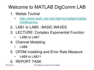
Welcome to MATLAB DigComm LAB. Matlab Toutrial http://www.math.utah.edu/lab/ms/matlab/matlab.html#starting LAB1 to LAB5 : BASIC WAVES LECTURE: Complex Exponential Function LAB6 to LAB7 Channel Modeling LAB8 OFDM modeling and Error Rate Measure LAB9 to LAB11 REPORT TASK. LAB1 : AM.

E N D
Welcome to MATLAB DigComm LAB • MatlabToutrial • http://www.math.utah.edu/lab/ms/matlab/matlab.html#starting • LAB1 to LAB5 : BASIC WAVES • LECTURE: Complex Exponential Function • LAB6 to LAB7 • Channel Modeling • LAB8 • OFDM modeling and Error Rate Measure • LAB9 to LAB11 • REPORT TASK 2013 DigComm Lab (Fire Tom Wada)
LAB1: AM • Write Amplitude Modulation (AM) program by MATLAB • A = 1 + 0.5*cos(2*pi*1*t) • fc =5Hz • Use Sampling frequency fs = 100Hz 2013 DigComm Lab (Fire Tom Wada)
LAB1: AM answer • n=0:1000; % 1001 points • fc=5; • fs=100; % Sampling Frequency • t = n/fs; % time index • % INPUT to Modulator • A = 1 + 0.5*cos(2*pi*1*t); • % OUTPUT • x = A .* sin(2*pi*fc*t); • % FIGURE • figure(1); • subplot(2,1,1); • plot(A); • subplot(2,1,2); • plot(x); 2013 DigComm Lab (Fire Tom Wada)
LAB2: AM Demodulation • Use LAB1 result x and calculate y as each x is squared. • If you connect each peak of y, you can recover original A. 2013 DigComm Lab (Fire Tom Wada)
LAB2:AM Demod answer • n=0:1000; % 1001 points • fc=5; • fs=100; % Sampling Frequency • t = n/fs; % time index • % INPUT to Modulator • A = 1 + 0.5*cos(2*pi*1*t); • % OUTPUT • x = A .* sin(2*pi*fc*t); • %% • y = x .* x; • % FIGURE • figure(2); • subplot(3,1,1); • plot(A); • subplot(3,1,2); • plot(x); • subplot(3,1,3); • plot(y); 2013 DigComm Lab (Fire Tom Wada)
0 1 0 1 0 1 0 1 LAB3: Spectrum of square wave • Analyze below pulse spectrum by Discrete Fourier Transform. 2013 DigComm Lab (Fire Tom Wada)
LAB3: Spectrum answer Assume T = 10 points • n=1:1:80; • x = [zeros(1,10), ones(1,10), zeros(1,10), ones(1,10), zeros(1,10), ones(1,10), zeros(1,10), ones(1,10)]; • figure(3) • subplot(2,1,1); • plot(x); • axis([1,80,-0.5, 1.5]); • %% • y = fft(x); • subplot(2,1,2); • plot(abs(y)); • axis([1,80,-10, 50]); 2013 DigComm Lab (Fire Tom Wada)
LAB4: BPSK waveform • Make BPSK waveformas follows When data=0 When data=1 2013 DigComm Lab (Fire Tom Wada)
LAB4:BPSK answer • n=0:32; • fc=2; • fs=32; % Sampling Frequency • t = n/fs; % time index • % BPSK waveform • x0 = cos(2*pi*fc*t); • x1 = cos(2*pi*fc*t + pi); • % FIGURE • figure(5); • subplot(2,1,1); • plot(x0); • subplot(2,1,2); • plot(x1); (A0, θ0)=(1, 0) (A1, θ1)=(1, π) 0 2013 DigComm Lab (Fire Tom Wada)
LAB5: QPSK waveform • Make QPSK waveformas follows (A0, Φ 0)=(1, 1π/4) (A1, Φ 1)=(1, 3π/4) 0 (A2, Φ 2)=(1, 5π/4) (A2, Φ 2)=(1, 7π/4) 2013 DigComm Lab (Fire Tom Wada)
LAB5:QPSK answer • n=0:32; • fc=2; • fs=32; % Sampling Frequency • t = n/fs; % time index • % QPSK waveform • x0 = cos(2*pi*fc*t + 1*pi/4); • x1 = cos(2*pi*fc*t + 3*pi/4); • x2 = cos(2*pi*fc*t + 5*pi/4); • x3 = cos(2*pi*fc*t + 7*pi/4); • % FIGURE • figure(5); • subplot(4,1,1); • plot(x0); • subplot(4,1,2); • plot(x1); • subplot(4,1,3); • plot(x2); • subplot(4,1,4); • plot(x3); 2013 DigComm Lab (Fire Tom Wada)
LECTURE:Complex Exponential Function 2013 DigComm Lab (Fire Tom Wada)
1. Complex Exponential Function • We will shift from SIN and COS toComplex Exponential Function. • Real and Imaginary =complex number • Real part is same as previous cosine wave. Real part Imaginary part 2013 DigComm Lab (Fire Tom Wada)
2. Real – Imaginary plane • IQplane • I: In-Phase = Real axis • Q: Quadrature-Phase = Imaginary axis • Real-Imaginary plane (Complex plane) • Complex number can be indicated as a point Imaginary axis (Q) Complex plane a + j b b Real axis (I) 0 a 2013 DigComm Lab (Fire Tom Wada)
Complex Exponential Function Shows Rotation in I-Q plane Real part Imaginary Imaginary (Q) A Real (I) 0 2013 DigComm Lab (Fire Tom Wada)
Complex Exponential Functionshows Rotation on TIME! 2013 DigComm Lab (Fire Tom Wada)
Complex Amplitude (Phaser) • X=x(t=0)showsstarting point (t=0) . • Xis called asComplex Amplitude (Phaser) 2013 DigComm Lab (Fire Tom Wada)
QPSK by Complex Exponential Function Imaginary (Q) Real (I) 0 Complex Amplitude (Phaser) = Constellation point 2013 DigComm Lab (Fire Tom Wada)
Conversion from Complex Exponential Functionto Real sinusoid. Take Real Part Then You can convert! 2013 DigComm Lab (Fire Tom Wada)
LAB6: QPSK waveform • Make QPSK waveformas follows using (A0, Φ 0)=(1, 1π/4) (A1, Φ 1)=(1, 3π/4) 0 (A2, Φ 2)=(1, 5π/4) (A2, Φ 2)=(1, 7π/4) 2013 DigComm Lab (Fire Tom Wada)
LAB6:QPSK (2) answer • n=0:32; fc=2; • fs=32; % Sampling Frequency • t = n/fs; % time index • % QPSK Phasers • X0 = exp(1j*1*pi/4); X1 = exp(1j*3*pi/4); • X2 = exp(1j*5*pi/4); X3 = exp(1j*7*pi/4); • % FIGURE • figure(61); plot([X0, X1, X2, X3], '+'); • axis([-1 1 -1 1]); • % • X0wave = X0 * exp(1j*2*pi*fc*t); X1wave = X1 * exp(1j*2*pi*fc*t); • X2wave = X2 * exp(1j*2*pi*fc*t); X3wave = X3 * exp(1j*2*pi*fc*t); • % • figure(62); • XX=real(X0wave); YY=imag(X0wave); ZZ=t; • plot3(XX, YY, ZZ); xlabel ('I'); ylabel('Q'); zlabel('time'); • % • figure(63); • subplot(4,1,1); plot(real(X0wave)); • subplot(4,1,2); plot(real(X1wave)); • subplot(4,1,3); plot(real(X2wave)); • subplot(4,1,4); plot(real(X3wave)); 2013 DigComm Lab (Fire Tom Wada)
LAB7: Draw BER graph • Make following graph by MATLAB 2013 DigComm Lab (Fire Tom Wada)
LAB7: BER graph answer • EBN0dB = 0:1:20; % EbN0 in dB • EBN0 = 10 .^(EBN0dB/10); • BER_QPSK = 0.5*erfc(sqrt(EBN0)); • figure(7); • semilogy(EBN0dB, BER_QPSK); • axis([0 20 1E-6 1]); • xlabel(' Eb/N0 (dB) '); • ylabel(' BER of OPSK'); • grid on; • title(' QPSK BER'); 2013 DigComm Lab (Fire Tom Wada)
LECTURE:Channel Modeling 2013 DigComm Lab (Fire Tom Wada)
Multipath Channel • Direct path and Delayed paths 2013 DigComm Lab (Fire Tom Wada)
Channel Modeling by Impulse Response H(z) Sending Signal Receiving Signal If sending signal is Impulse then, Received signal has many delayed components. This outputs shows CHANEL IMPULSE RESPONSE 2013 DigComm Lab (Fire Tom Wada)
Convolution operation • If you multiply two polynomial • Channel Impulse Response=(1, 0.5, 0.2) • Send (1, 1, 1, 1, 1) signal • Then Received Signal is (1,1.5,1.7,1.7,1.7,0.7,0.2) 2013 DigComm Lab (Fire Tom Wada)
Channel Modeling by Impulse Response H(z) Sending Signal Receiving Signal (1,1.5,1.7,1.7,1.7,0.7,0.2) (1, 1, 1, 1, 1) H(z) =(1, 0.5, 0.2) This can be calculated by CONVOLUTION. 2013 DigComm Lab (Fire Tom Wada)
LAB8: CHANNEL • Assume Channel Impulse Response =(1, 0.5, 0.2) • Show each received signal for • x1 = [1,0,0,0,0,0,0]; • x2 = [1,1,1,1,1,0,0]; • n = 1:100; x3 = cos(2*pi*n/32); 2013 DigComm Lab (Fire Tom Wada)
LAB8: CHANNEL answer • %% CHANNEL • h = [1, 0.5, 0.2]; • %% INPUT signal 1 • x1 = [1,0,0,0,0,0,0]; • y1 =conv(h, x1); % OUTPUT signal • figure(81)% FIGURE • xa=1:7; • subplot(2,1,1); stem(xa, x1(1:7)); title('TX'); • subplot(2,1,2); stem(xa, y1(1:7)); title('RX'); • %% INPUT signal 2 • x2 = [1,1,1,1,1,0,0]; • y2 =conv(h, x2); % OUTPUT signal • figure(82)% FIGURE • xa=1:7; • subplot(2,1,1); stem(xa, x2(1:7)); title('TX'); • subplot(2,1,2); stem(xa, y2(1:7)); title('RX'); • %% INPUT signal 3 • n = 1:100; x3 = cos(2*pi*n/32); • y3 =conv(h, x3);% OUTPUT signal • figure(83)% FIGURE • xa=1:100; • subplot(2,1,1); stem(xa, x3(1:100)); title('TX'); • subplot(2,1,2); stem(xa, y3(1:100)); title('RX'); 2013 DigComm Lab (Fire Tom Wada)
LECTURE:OFDM Modeling 2013 DigComm Lab (Fire Tom Wada)
Q 00 01 I 11 10 OFDM digital communication WORK SHEET u3 We are going to send 8bits by the following OFDM communication system ④ GIadd u3 u0 u1 u2 u3 u0 u0 00 d0=1+j ① ② MAP ③ I F F T u1 u1 d1=-1+j 01 00011011 u2 u2 d2=1-j 10 GI OFDM u3 u3 11 d3=-1-j u3 ⑤ GIrmv d0=1+j u0 u0 00 ⑥ F F T ⑦ DeMAP ⑧ d1=-1+j u1 u1 01 00011011 d2=1-j u2 u2 10 d3=-1-j u3 u3 11 2013 DigComm Lab (Fire Tom Wada)
LAB9 OFDM • Please draw OFDM symbol complex wave form including GI when you send “00011011”. • Please draw OFDM symbol complex wave form including GI when you send “10010011”. • Please draw OFDM symbol complex wave form including GI when you send “00000000”. • Compare those 3 waveform. Then Did you find any problem? If yes, please state the problem. Effective Symbol I GI Time Q Time 2013 DigComm Lab (Fire Tom Wada)
LAB9 1) answer • %% • data=[0,1,2,3]; % 0->00, 1->01, 2->10, 3->11 • % MAP • modqpsk= [1+i, -1+i, 1-i, -1-i]; • const =modqpsk(data+1); • % IFFT • uu = ifft(const); • % GI ADD • uu_g =[uu(4), uu]; • % FIGURE • figure(81) • subplot(3,1,1); plot(real(uu_g),'*-'); axis([1 5 -2 2]); • subplot(3,1,2); plot(imag(uu_g),'*-'); axis([1 5 -2 2]); • subplot(3,1,3); plot(abs(uu_g),'*-'); axis([1 5 -2 2]); 2013 DigComm Lab (Fire Tom Wada)
LAB10 OFDM MAKE 100 symbol OFDM signal based on previous 4 point OFDM + 1 point GI. Add noise of SNR=10dB 2013 DigComm Lab (Fire Tom Wada)
LAB10 OFDM answer • % Simple OFDM system (send 8 bits/symbol * 100 symbol) • % Fire Wada • clear all; • num_symbol = 100; % number of symbols • n_symbol = 4; % points in symbol • M = 4; % size of signal constellation • modqpsk= [1+i, -1+i, 1-i, -1-i]; • %% 1 . create random data • data = floor(rand(n_symbol,num_symbol)*M); • %% 2. mapping into I-Q constellation • data_1 = modqpsk(1+data); • figure(100); • subplot(2,2,1); • plot(data_1,'r.'); • axis([-3 3 -3 3]) • title('data constellation') • data_2 = data_1; • %% 3. IFFT • data_3 = ifft(data_2); • subplot(2,2,2); • plot((real(data_3)),'-'); • title('IFFT'); • %% 4. GI add • data_4 = [data_3(n_symbol,:);data_3]; • %%4.1 Add Noise • sigpower=mean(mean(abs(data_4).^2)); • sn= 10; %% 10dB • awgn = (randn(n_symbol+1,num_symbol)+i*randn(n_symbol+1,num_symbol)); • awgnpower=mean(mean(abs(awgn).^2)); • awgn = awgn/sqrt(awgnpower)*10^(-sn/20)*sqrt(sigpower); • data_4=data_4+awgn; • subplot(2,2,3); • plot(real(data_4),'-'); • title('GI add'); • %% 5. GI remove • data_5 = data_4(2:n_symbol+1,:); • %% 6. FFT • data_6 = fft(data_5); • subplot(2,2,4); • plot(data_6,'b.'); • axis([-3 3 -3 3]) • title('receive data constellation') • figure(200) • plot(real(reshape(data_4,(n_symbol+1)*num_symbol,1))); 2013 DigComm Lab (Fire Tom Wada)
LAB10 OFDM answer 2013 DigComm Lab (Fire Tom Wada)
LAB11 Symbol Error Rate Measure Symbol Error Rate for LAB10. Add noise of SNR=0dB, 5dB, 10dB. Use ‘demapQPSK.m’ function. Put the m-file in same directory. % demapQPSK.m % The program demap to Complex to Numerical data. function graycode = demapQPSK(comp) re = real(comp); im = imag(comp); if (re >= 0 & im >= 0 ) graycode=0; elseif (re < 0 & im >= 0 ) graycode=1; elseif (re >= 0 & im < 0 ) graycode=2; else graycode=3; end 2013 DigComm Lab (Fire Tom Wada)
LAB11 Symbol Error Rate • % Simple OFDM system (send 8 bits/symbol * 100 symbol) • % Fire Wada • clear all; • num_symbol = 100; % number of symbols • n_symbol = 4; % points in symbol • M = 4; % size of signal constellation • modqpsk= [1+i, -1+i, 1-i, -1-i]; • %% 1 . create random data • data = floor(rand(n_symbol,num_symbol)*M); • %% 2. mapping into I-Q constellation • data_1 = modqpsk(1+data); • data_2 = data_1; • %% 3. IFFT • data_3 = ifft(data_2); • %% 4. GI add • data_4 = [data_3(n_symbol,:);data_3]; • %%4.1 Add Noise • sigpower=mean(mean(abs(data_4).^2)); • sn= 5; %% 10dB • awgn = (randn(n_symbol+1,num_symbol)+i*randn(n_symbol+1,num_symbol)); • awgnpower=mean(mean(abs(awgn).^2)); • awgn = awgn/sqrt(awgnpower)*10^(-sn/20)*sqrt(sigpower); • data_4=data_4+awgn; • %% 5. GI remove • data_5 = data_4(2:n_symbol+1,:); • %% 6. FFT • data_6 = fft(data_5); • figure(11) • plot(data_6,'b.'); • axis([-3 3 -3 3]) • title('receive data constellation') • %% 7. recover data • rdata=zeros(n_symbol,num_symbol); • for sym = 1: num_symbol • for index = 1:n_symbol • rdata(index, sym) = demapQPSK(data_6(index,sym)); • end • end • %% 8. measure Symbol Error Rate by compare data and rdata • Total_data= n_symbol*num_symbol; • diff = rdata - data; • % count how many not zero in diff • notZero = (diff ~= 0); • Total_error=sum(sum(notZero)); • fprintf('*** SNR =%4.2f, *** SYMBOL ERROR RATE = %8.5f *** \n', sn, Total_error/Total_data); 2013 DigComm Lab (Fire Tom Wada)
TASK1 • Make a Matlab program to measure Symbol Error Rate vsSN ratioin 1K OFDM with QPSK modulation • FFT size = 1024 points in 1 symbol • GI length = 1/8*FFT size = 128 points • Total 100 symbol • Write Mid Report to explain OFDM simulation including • Your Matlab program • Total 100 symbol waveform • Consternation with SNR=0, 3, 6, 9dB • Symbol Error Rate vsSNR Graph • Vertical: SER in log scale • Horizontal: SN ratio 0dB, 1dB … to 10dB 2013 DigComm Lab (Fire Tom Wada)