Download
1 / 51
530 likes | 707 Views
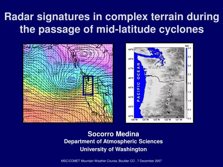
Radar signatures in complex terrain during the passage of mid-latitude cyclones. Socorro Medina Department of Atmospheric Sciences University of Washington. MSC/COMET Mountain Weather Course, Boulder CO , 7 December 2007. Observational Perspective Field Experiments.

E N D
Radar signatures in complex terrain during the passage of mid-latitude cyclones Socorro Medina Department of Atmospheric Sciences University of Washington MSC/COMET Mountain Weather Course, Boulder CO , 7 December 2007
Observational Perspective Field Experiments • “MAP” – Mesoscale Alpine Programe • “IMPROVE-2” – Second phase of the Improvement of Microphysical PaRameterization through Observation Verification Experiment
MAPEuropean AlpsSeptember-November 1999 500-mb geopotential height (black lines) and temperature (shaded) Orography
IMPROVE-2Oregon Cascade MountainsNovember-December 2001 500-mb geopotential height (black lines) and temperature (shaded) Orography
Synoptic conditions of MAP and IMPROVE-2 storms:◘ Baroclinic system approaching orographic barrier ◘ Flow far upstream nearly perpendicular to terrain
NOAA WP-3D MAP and IMPROVE-2 radar observations Mean crest = 2 km MSL Mean crest = 3 km MSL S-Pol = NCAR S-band polarimetric radar
Range-Height Indicator (RHI) Fix the azimuth and scan in elevation Radar scanning modes range Horizontal distance Vertical distance range Azimuth (fixed) Elevation (scan) Horizontal distance Horizontal distance RADAR RADAR
Range-Height Indicator (RHI) Fix the azimuth and scan in elevation Radar scanning modes range Horizontal distance Vertical distance Azimuth (fixed) Horizontal distance Horizontal distance RADAR RADAR
Plan Position Indicator (PPI): Fix the elevation angle and scan in azimuth Radar scanning modes range Horizontal distance Vertical distance range Azimuth (scan) (Elevation fixed) Horizontal distance Horizontal distance RADAR RADAR
Plan Position Indicator (PPI): Fix the elevation angle and scan in azimuth Radar scanning modes Horizontal distance Vertical distance range (Elevation fixed) Horizontal distance Horizontal distance RADAR RADAR
Radar measurements • Reflectivity factor (often called reflectivity): Quantity proportional to the sixth-power of the diameters of all the raindrops in a unit volume • Radial velocity: The flow component in the direction of the radar beam
Methodology: Time-averaged vertical cross-sections (from RHI data) MAP IMPROVE-2
Mean Radial velocity (m s-1; from RHIs) Type A low-level flow rises over terrain MAP Case (IOP2b, 3-hour mean) IMPROVE-2 Case (IOP6, 2-hour mean) NNW E S-POL S-POL
Mean Radial velocity (m s-1; from RHIs) Type B low-level flow doesn’t rise over terrain ; shear layer MAP (IOP8, 3-hour S-Pol mean) IMPROVE-2 (IOP1, 3-hour mean) E S-POL NNW S-POL
IOP8 (Type B) Airborne radar-derived low-level winds Bousquet and Smull (2006)
IOP8 (Type B) Airborne radar-derived down valley flow Bousquet and Smull (2003)
Summary of terrain-modified airflow in MAP and IMPROVE-2 storms:◘ Type A: Low-level jet rises over the first peaks of the terrain◘ Type B: Shear layer rises over terrain
Measure of stability in moist flow moist Brunt-Vaisala frequency to include latent heating effects (Durran and Klemp, 1982)
Type A cases stability profiles STABLE UNSTABLE
Type B cases stability profiles STABLE UNSTABLE
Summary of static stability in MAP and IMPROVE-2 storms: ◘ Type A: Potential instability ◘ Type B: Statically stable
Mean Reflectivity (dBZ) Type A Maximum over first major peak MAP Case (IOP2b, 3-hour mean) IMPROVE-2 Case (IOP6, 2-hour mean) NNW E S-POL S-POL
Mean Reflectivity (dBZ) Type B Bright band MAP Case (IOP8, 3-hour mean) IMPROVE-2 Case (IOP1, 3-hour mean) NW E S-POL S-POL
Summary of reflectivity patterns in MAP and IMPROVE-2 storms:◘ Type A: Localized maximum on terrain peak ◘ Type B: Bright band
cloud droplets graupel growing by riming rain growing by coalescence snow rain Slightly unstable air TYPE A conceptual model of precipitation enhancement for flow rising over terrain 0ºC Low static stability TERRAIN Medina and Houze (2003) Medina and Houze (2003)
Small-scale cells in Type B (Case 01) Vertically pointing radar
Region of enhanced growth by riming and aggregation Region of enhanced growth by coalescence TYPE B conceptual Model of precipitation enhancement for cases with statically stable and retarded low-level flow Shear layer and overturning cells 0°C SNOW RAIN OVERTURNING CELLS Houze and Medina (2005)
Results shown so far from RHI scans, but RHIs are not available in operational scanning - What do Type A and B flow structures look like in PPIs?
Range Z1 < Z2 PPI range as a proxy of height
Orography (km) 4.0 Ticino 3.5 Toce 3.0 2.5 S-Pol 2.0 32 Sounding 24 1.5 16 1.0 Po Basin 8 0.5 0 0.0 -8 -16 -24 -32 Radial velocity (m s-1); PPI = 3.8° Type A case MAP IOP2b 10 UTC 20 Sep (b)
Orography (km) 4.0 Ticino 3.5 Toce 3.0 2.5 S-Pol 2.0 32 Sounding 24 1.5 16 1.0 Po Basin 8 0.5 0 0.0 -8 -16 -24 -32 Radial velocity (m s-1); PPI = 3.8° Type A case MAP IOP2b 10 UTC 20 Sep (b)
MAP Case (IOP2b, 3-hour mean) 32 24 NNW S-POL 16 8 0 -8 -16 -24 -32 Radial velocity (m s-1); PPI = 3.8° Type A case MAP IOP2b 10 UTC 20 Sep Range < 20 km Height < 1.5 km MSL
Orography (km) 4.0 Ticino 3.5 Toce 3.0 2.5 S-Pol 2.0 32 Sounding 24 1.5 16 1.0 Po Basin 8 0.5 0 0.0 -8 -16 -24 -32 Radial velocity (m s-1); PPI = 3.8° Type A case MAP IOP2b 10 UTC 20 Sep (b)
500-mb geopotential height (black lines) and temperature12 UTC 20 Sep 32 24 16 8 0 -8 -16 -24 -32 Radial velocity (m s-1); PPI = 3.8° Type A case MAP IOP2b 10 UTC 20 Sep 30 km < Range < 70 km 2 km < Height < 5 km MSL (b)
4.0 Ticino 3.5 Toce 3.0 2.5 S-Pol 2.0 32 Sounding 24 1.5 16 1.0 Po Basin 8 0.5 0 0.0 -8 -16 -24 -32 Orography (km) Radial velocity (m s-1); PPI = 3.8° Type B case MAP IOP8 06 UTC 21 Oct
4.0 Ticino 3.5 Toce 3.0 2.5 S-Pol 2.0 32 Sounding 24 1.5 16 1.0 Po Basin 8 0.5 0 0.0 -8 -16 -24 -32 Orography (km) Radial velocity (m s-1); PPI = 3.8° Type B case MAP IOP8 06 UTC 21 Oct (b)
MAP (IOP8, 3-hour S-Pol mean) 32 24 16 8 NNW S-POL 0 -8 -16 -24 -32 Radial velocity (m s-1); PPI = 3.8° Type B case MAP IOP8 06 UTC 21 Oct (b) Range < 10 km Height < 1 km MSL
MAP (IOP8, 3-hour S-Pol mean) 32 24 16 8 NNW S-POL 0 -8 -16 -24 -32 Radial velocity (m s-1); PPI = 3.8° Type B case MAP IOP8 06 UTC 21 Oct 20 km < Range < 30 km 1.5 km < Height < 2 km MSL Mid-level flow
32 24 16 8 0 -8 -16 -24 -32 Orography (km) Radial velocity (m s-1); PPI = 3.8° Type B case MAP IOP8 06 UTC 21 Oct 20 km < Range < 30 km 1.5 km < Height < 2 km MSL (b) Mid-level flow
32 24 16 8 0 -8 -16 -24 -32 500-mb geopotential height (black lines) and temperature06 UTC 21 Oct Radial velocity (m s-1); PPI = 3.8° Type B case MAP IOP8 06 UTC 21 Oct 30 km < Range < 70 km 2 km < Height < 5 km MSL
4.0 Ticino 3.5 Toce 3.0 2.5 S-Pol 2.0 32 Sounding 24 1.5 16 1.0 Po Basin 8 0.5 0 0.0 -8 -16 -24 -32 Orography (km) Radial velocity (m s-1); PPI = 3.8° Type B case MAP IOP8 06 UTC 21 Oct
u p p e r – l e v e l f l o w cross-barrier flow low-level flow Using flows below 5 km (from PPI scans) for nowcasting of precipitation Low-Level Flow : 1.5 - 2 km height over the closest plane Cross-Barrier Flow: 2.5 - 3.5 km height just South of the Alpine crest Upper-Level Flow: 4 - 5 km height in a circle Work by Panziera and Germann 2007 (MeteoSwiss)
Using flows below 5 km (from PPI scans) for nowcasting of precipitation A decrease of the three flows intensities seems to anticipate the end of the heavy rain. Magnitude (m/s) Rain (averaged over several basins) Panziera and Germann (2007)
Conclusions • -Two predominant terrain-modified flow patterns during orographic enhancement of precipitation have been identified (Types A and B) • -Both patterns produce strong updrafts (>2m/s) • -During Type A cases static instability is responsible for the updraft generation versus turbulent instability in Type B • -During both Types the enhancement of precipitation is produced by the accretion processes (coalescence, aggregation and riming) • -The flows at low-levels have some potential for nowcasting precipitation
16 March 2007 Whistler case TYPE B case (MAP IOP8)