Download
1 / 13
140 likes | 155 Views
FluxEs: An R package for metabolic flux quantification. Thomas Binsl http://www.few.vu.nl/~tbinsl. Introduction. Metabolic fluxes reflect the function and dynamics of living cells.

E N D
FluxEs: An R package for metabolic flux quantification Thomas Binsl http://www.few.vu.nl/~tbinsl
Introduction • Metabolic fluxes reflect the function and dynamics of living cells. • A number of new techniques for flux measurement have been developed, which aids for instance dedicated drug development and the design of new efficient bioreactors. • FluxEs is an R computer package that quantifies metabolic fluxes using NMR measurements of isotope labeling experiments. • User-/biologist-friendly input format. • No isotope steady state necessary.
A B v v D C v Isotope Labeling Experiment A B v v C2 C3 C1 C2 D C1 v C C1 v C2 v C1
Parameter Estimation • By performing a computer simulation of the labeling experiment the NMR multiplets can also be computed… • …and model parameters, like the cycle flux v can be esti-mated by comparing the computed and measured NMR multiplets, e.g. via sum of squares (SSQ) criterion.
Why R? • Free of charge • Cross platform, e.g. FluxEs was developed on a MS Windows machine and runs without any changes on our Linux cluster. • Object oriented • Vector based • Large variety of additional packages, e.g. FluxEs uses the “deSolve” package for solving the initial value problem for stiff systems of ordinary differential equations.
Program Implementation • Models are specified in plain text files. • The model-files are parsed by the package and the mathematical representation of the model is derived automatically. • Afterwards, the user is guided through the entire setup process necessary for an optimization, e.g. which parameters should be optimized, which optimization strategy should be used,…
Optimization Strategy • New grid-polyhedron approach to determine optimal start points for an optimization in parameter space. • Here we see a contour plot of sum-of-squares (SSQ) landscape formed by two parameters p1 and p2. • Grid points are the vertices of polyhedrons. • SSQ values of the vertices of a polyhedron are averaged and serve as SSQ value of the entire polyhedron. • Polyhedrons are sorted according to these values and the n best are chosen. • For each of the n polyhedrons the best vertex is used as start point for a global parameter estimation. • Additional start points are the n center points and the n best grid points. p2 p1
Results • Excellent agreement between the computed oxygen consumptions and the 'gold standard‘. • Oxygen consumption with the 'gold standard' method is determined for a much larger area than with the isotope labeling method, but the physiological condition in both areas are the same. • Although biological differences between the areas measured and not measured with the isotope labeling method (both included in the blood gas measurement) undoubtedly contribute to deviations from the line of identity, the general correspondence is still surprisingly good.
Acknowledgements • Hans van Beek • David Alders • Anne-Christin Hauschild • Entire IBIVU Group
Optimization Strategy (Random Start Points) Noisy data 1 Noisy data 2 . . . . Noisy data 25 30 best (of each data set) used for re-estimation of true parameter values 10,000 random start values for each noisy data set Syntheticdata
Optimization Strategy (Grid-Polyhedron) Noisy data 1 Noisy data 2 . . . . Noisy data 25 30 start points (for each data set) generated using the grid-polyhedron approach. Syntheticdata