Download

1 / 63
630 likes | 1.02k Views
Timing Analysis and Timing Predictability Reinhard Wilhelm Saarbrücken. Structure of the Talk. Timing Analysis – the Problem Timing Analysis – our Solution the overall approach, tool architecture cache analysis Results and experience The influence of Software

E N D
Timing Analysis and Timing Predictability Reinhard WilhelmSaarbrücken
Structure of the Talk • Timing Analysis – the Problem • Timing Analysis – our Solution • the overall approach, tool architecture • cache analysis • Results and experience • The influence of Software • Design for Timing Predictability • predictability of cache replacement strategies • Conclusion
Sideairbag in car, Reaction in <10 mSec Wing vibration of airplane, sensing every 5 mSec Industrial Needs Hard real-time systems, often in safety-critical applications abound • Aeronautics, automotive, train industries, manufacturing control
Hard Real-Time Systems • Embedded controllers are expected to finish their tasks reliably within time bounds. • Task scheduling must be performed • Essential: upper bound on the execution times of all tasks statically known • Commonly called theWorst-Case Execution Time (WCET) • Analogously, Best-Case Execution Time (BCET)
Modern Hardware Features • Modern processors increase performance by using: Caches, Pipelines, Branch Prediction, Speculation • These features make WCET computation difficult:Execution times of instructions vary widely • Best case - everything goes smoothely: no cache miss, operands ready, needed resources free, branch correctly predicted • Worst case - everything goes wrong: all loads miss the cache, resources needed are occupied, operands are not ready • Span may be several hundred cycles
Timing Accidents and Penalties Timing Accident – cause for an increase of the execution time of an instruction Timing Penalty – the associated increase • Types of timing accidents • Cache misses • Pipeline stalls • Branch mispredictions • Bus collisions • Memory refresh of DRAM • TLB miss
How to Deal with Murphy’s Law? Essentially three different answers: • Accepting: Every timing accident that may happen will happen • Fighting: Reliably showing that many/most Timing Accidents cannot happen • Cheating: monitoring “enough” runs to get a good feeling
Accepting Murphy’s Law like guaranteeing a speed of 4.07 km/h for this car because variability of execution times on modern processors is in the order of 100
Cheating to deal with Murphy’s Law • measuring “enough” runs to feel comfortable • how many runs are “enough”? • Example: Analogy – Testing vs. VerificationAMD was offered a verification of the K7.They had tested the design with 80 000 test vectors, considered verification unnecessary.Verification attempt discovered 2 000 bugs! The only remaining solution: Fighting Murphy’s Law!
Execution Time is History-Sensitive Contribution of the execution of an instruction to a program‘s execution time • depends on the execution state, i.e., on the execution so far, • i.e., cannot be determined in isolation • history sensitivity is not only a problem – it’s also a chance!
Deriving Run-Time Guarantees • Static Program Analysis derives Invariants about all execution states at a program point. • Derive Safety Properties from these invariants : Certain timing accidents will never happen.Example:At program point p, instruction fetch will never cause a cache miss. • The more accidents excluded, the lower the upper bound. • (and the more accidents predicted, the higher the lower bound).
Worst-case guarantee Lower bound Upper bound t Worst case Best case Basic Notions
Overall Approach: Natural Modularization • Processor-Behavior Analysis: • Uses Abstract Interpretation • Excludes as many Timing Accidents as possible • Determines upper bound for basic blocks (in contexts) • Bounds Calculation • Maps control flow graph to an integer linear program • Determines upper bound and associated path
Executable program Path Analysis AIP File CRL File PER File Loop bounds WCET Visualization Loop Trafo LP-Solver ILP-Generator CFG Builder Evaluation Value Analyzer Cache/Pipeline Analyzer Overall Structure Static Analyses Processor-Behavior Analysis Bounds Calculation
Static Program Analysis Applied to WCET Determination • Upper bounds must be safe, i.e. not underestimated • Upperbounds should be tight, i.e. not far away from real execution times • Analogous for lower bounds • Effort must be tolerable
Abstract Interpretation (AI) • semantics-based method for static program analysis • Basic idea of AI: Perform the program's computations using value descriptions or abstract valuesin place of the concrete values, start with a description of all possible inputs • AI supports correctness proofs • Tool support (Program-Analysis Generator PAG)
Abstract Interpretation – the Ingredients and one Example • abstract domain – complete semilattice,related to concrete domain by abstraction and concretization functions, e.g. intervals of integers (including -, ) instead of integer values • abstract transfer functions for each statement type – abstract versions of their semantics e.g. arithmetic and assignment on intervals • a join function combining abstract values from different control-flow paths – lub on the latticee.g. “union” on intervals • Example: Interval analysis (Cousot/Halbwachs78)
Value Analysis • Motivation: • Provide access information to data-cache/pipeline analysis • Detect infeasible paths • Derive loop bounds • Method: calculate intervals, i.e. lower and upper bounds, as in the example abovefor the values occurring in the machine program (addresses, register contents, local and global variables)
Value Analysis II D1: [-4,4], A[0x1000,0x1000] move.l #4,D0 • Intervals are computed along the CFG edges • At joins, intervals are „unioned“ D0[4,4], D1: [-4,4], A[0x1000,0x1000] add.l D1,D0 D0[0,8], D1: [-4,4], A[0x1000,0x1000] D1: [-2,+2] D1: [-4,0] D1: [-4,+2] move.l (A0,D0),D1 Which address is accessed here? access[0x1000,0x1008]
Value Analysis (Airbus Benchmark) 1Ghz Athlon, Memory usage <= 20MB Good means less than 16 cache lines
Caches: Fast Memory on Chip • Caches are used, because • Fast main memory is too expensive • The speed gap between CPU and memory is too large and increasing • Caches work well in the average case: • Programs access data locally (many hits) • Programs reuse items (instructions, data) • Access patterns are distributed evenly across the cache
Caches: How the work CPU wants to read/write at memory address a,sends a request for a to the bus Cases: • Block m containing a in the cache (hit): request for a is served in the next cycle • Blockm not in the cache (miss):m is transferred from main memory to the cache, m may replace some block in the cache,request for a is served asap while transfer still continues • Several replacement strategies: LRU, PLRU, FIFO,...determine which line to replace
Address prefix Set number Byte in line A-Way Set Associative Cache CPU Address: Compare address prefix If not equal, fetch block from memory Main Memory Byte select & align Data Out
Cache Analysis How to statically precompute cache contents: • Must Analysis:For each program point (and calling context), find out which blocks are in the cache • May Analysis: For each program point (and calling context), find out which blocks may be in the cacheComplement says what is not in the cache
Must-Cache and May-Cache- Information • Must Analysis determines safe information about cache hitsEach predicted cache hit reduces upper bound • May Analysis determines safe information about cache missesEach predicted cache miss increases lower bound
concrete (processor) “young” z y x t s z y x Age “old” s z x t z s x t [ s ] abstract (analysis) { s } { x } { t } { y } { x } { } { s, t } { y } [ s ] Cache with LRU Replacement: Transfer for must LRU has a notion of AGE
{ a } { } { c, f } { d } { c } { e } { a } { d } “intersection + maximal age” { } { } { a, c } { d } Cache Analysis: Join (must) Join (must) Interpretation: memory block a is definitively in the (concrete) cache => always hit
concrete “young” z y x t s z y x Age “old” s z x t z s x t [ s ] abstract { s } { x } { } {y, t } { x } { } {s, t } { y } [ s ] Cache with LRU Replacement: Transfer for may
{ a } { } { c, f } { d } { c } { e } { a } { d } “union + minimal age” { a,c } { e} { f } { d } Cache Analysis: Join (may) Join (may)
Penalties for Memory Accesses(in #cycles for PowerPC 755) Penalties have to be assumed for uncertainties! Tendency increasing, since clocks are getting faster faster than everything else
Cache Impact of Language Constructs • Pointer to data • Function pointer • Dynamic method invocation • Service demultiplexing CORBA
The Cost of Uncertainty Cost of statically unresolvable dynamic behavior. Basic idea: What does it cost me if I cannot exclude a timing accident? This could be the basis for design and implementation decisions.
{ } { x } { } {s, t } { x } { } { s, t} { y } Cache with LRU Replacement: Transfer for must under unknown access, e.g. unresolved data pointer Set of abstract cache [ ? ] If address is completely undetermined, same loss and no gain of information in every cache set! Analogously for multiple unknown accesses, e.g. unknown function pointer; assume maximal cache damage
Dynamic Method Invocation • Traversal of a data structure representing the class hierarchy • Corresponding worst-case execution time and resulting cache damage • Efficient implementation [WiMa] with table lookup needs 2 indirect memory references; if page faults cannot be excluded: 2 x pf = 4000 cycles!
Fetch Decode Execute WB Fetch Decode Execute Execute Fetch WB WB Decode Fetch Decode WB Execute Pipelines Inst 1 Inst 3 Inst 2 Inst 4 Fetch Decode Execute WB Ideal Case: 1 Instruction per Cycle
Pipeline Hazards Pipeline Hazards: • Data Hazards: Operands not yet available (Data Dependences) • Resource Hazards: Consecutive instructions use same resource • Control Hazards: Conditional branch • Instruction-Cache Hazards: Instruction fetch causes cache miss
More Threats • Out-of-order execution • Speculation • Timing Anomalies Consider all possible execution orders ditto Considering the locally worst-case path insufficent
CPU as a (Concrete) State Machine • Processor (pipeline, cache, memory, inputs) viewed as a bigstate machine, performing transitions every clock cycle • Starting in an initial state for an instruction transitions are performed, until a final state is reached: • End state: instruction has left the pipeline • # transitions: execution time of instruction
A Concrete Pipeline Executing a Basic Block function exec (b : basic block, s : concrete pipeline state) t: trace interprets instruction stream of b starting in state s producing trace t. Successor basic block is interpreted starting in initial state last(t) length(t) gives number of cycles
An Abstract Pipeline Executing a Basic Block functionexec (b : basic block, s : abstract pipeline state) t: trace interprets instruction stream of b (annotated with cache information) starting in state s producing trace t length(t) gives number of cycles
s2 s1 s? What is different? • Abstract states may lack information, e.g. about cache contents. • Assume local worst cases is safe(in the case of no timing anomalies) • Traces may be longer (but never shorter). • Starting state for successor basic block? In particular, if there are several predecessor blocks. • Alternatives: • sets of states • combine by least upper bound
s1 s3 s2 s1 Basic Block s10 s13 s11 s12 Integrated Analysis: Overall Picture Fixed point iteration over Basic Blocks (in context) {s1, s2, s3}abstract state Cyclewise evolution of processor modelfor instruction s1s2s3 move.1 (A0,D0),D1
How to Create a Pipeline Analysis? • Starting point: Concrete model of execution • First build reduced model • E.g. forget about the store, registers etc. • Then build abstract timing model • Change of domain to abstract states,i.e. sets of (reduced) concrete states • Conservative in execution times of instructions
Defining the Concrete State Machine How to define such a complex state machine? • A state consists of (the state of) internal components (register contents, fetch/ retirement queue contents...) • Combine internal components into units (modularisation, cf. VHDL/Verilog) • Units communicate via signals • (Big-step) Transitions via unit-state updates and signalsends and receives
An Example: MCF5307 • MCF 5307 is a V3 Coldfire family member • Coldfire is the successor family to the M68K processor generation • Restricted in instruction size, addressing modes and implemented M68K opcodes • MCF 5307: small and cheap chip with integrated peripherals • Separated but coupled bus/core clock frequencies
ColdFire Pipeline The ColdFire pipeline consists of • a Fetch Pipeline of 4 stages • Instruction Address Generation (IAG) • Instruction Fetch Cycle 1 (IC1) • Instruction Fetch Cycle 2 (IC2) • Instruction Early Decode (IED) • an Instruction Buffer (IB) for 8 instructions • an Execution Pipeline of 2 stages • Decoding and register operand fetching (1 cycle) • Memory access and execution (1 – many cycles)
Two coupled pipelines • Fetch pipeline performs branch prediction • Instruction executes in up two to iterations through OEP • Coupling FIFO buffer with 8 entries • Pipelines share same bus • Unified cache
Hierarchical bus structure • Pipelined K- and M-Bus • Fast K-Bus to internal memories • M-Bus to integrated peripherals • E-Bus to external memory • Busses independent • Bus unit: K2M, SBC, Cache
Concrete State Machine Abstract Model Model with Units and Signals Opaque components - not modeled: thrown away in the analysis (e.g. registers up to memory accesses) Reduced Model Opaque Elements Units & Signals Abstraction of components