Download

1 / 33
330 likes | 571 Views
Multi-view matching for unordered image sets. Abbas Roayaei. Multi-view matching for unordered image sets. Problem : establishing relative viewpoints given a large number of images where no ordering information is provided

E N D
Multi-view matching for unordered image sets Abbas Roayaei
Multi-view matching for unordered image sets • Problem: establishing relative viewpoints given a large number of images where no ordering information is provided • Application: images are obtained from different sources or at different times
Multi-view matching for unordered image sets • Given an unordered set of images, divide the data into clusters of related (i.e. from the same scene) images and determine the viewpoints of each image -> spatially organizing the image set
Image set example • The image set may have been acquired by a person photographing a scene (e.g. a castle or mountain) at various angles while walking back and forth around the area • The set may be the response from a query to an image database (e.g. a web search engine)
We develop an efficient indexing scheme based on invariant image patches • The output is a table of features vsviews • The table at this stage will contain many ambiguous and many erroneous matches. • The overall complexity of this stage is linear in the number of images.
The quality of the matches is improved by a number of global “clean-up” operations such as selective use of two-view and three-view matching constraints. • The output is a feature vs view table with considerably more correct matches, and fewer incorrect matches. • The complexity of this stage, which is opportunistic, is linear in the number of views
A 3D reconstruction of cameras and points is computed for connected sub-sets of views using the multiple view tracks
From images to multiview matches • Objective: efficiently determine putative multiple view matches, i.e. a point correspondence over multiple images. • Features with viewpoint invariant descriptors • affine geometric transformation • affine photometric transformation • Features are determined in two stages: • regions which transform covariantlywith viewpoint in each image • a vector of invariant descriptors is computed for each region • The invariant vector is a label for that region, and will be used as an index into an indexing structure for matching between views using the fact that: • The corresponding region in other images will (ideally) have an identical vector.
These features are determined in all images independently. • The descriptors for all images are then stored in the indexing structure. • Features with ‘close’ descriptors establish a putative multiple view match.
Covariant regions • We use two types of features: • based on interest point neighborhoods. • based on the “Maximally Stable Extremal” (MSE) regions • Each feature defines an elliptical (viewpoint covariant) region which is used to construct an invariant descriptor
Interest point neighborhood: generally succeeds at points where there is signal variation in more than one direction (e.g. near “blobs” or “corners”) • MSE regions: typically correspond to blobs of high contrast with respect to their surroundings.
Invariant descriptor • Apply a bank of linear filters, Kmn, similar to derivatives of a Gaussian • Taking the absolute value of each filter response gives 16 invariants • Using this formula we guarantee that Euclidean distance in invariant space is a lower bound on image SSD difference
Find, among the coefficients for with the one with the largest absolute value and artificially “rotate” the patch so as to make the phase zero. • We have constructed, for each neighborhood, a feature vector which is invariant to affine intensity and image transformations.
Invariant indexing • By comparing the invariant vectors for each point over all views, potential matches may be hypothesized • The query that we wish to support is “find all points within distance of this given point”. • Use a binary space partition tree, for finding matches
Verification • Since two different patches may have similar invariant vectors, a “hit” match does not mean that the image regions are affine related -> we need a verification step • Two points are deemed matched if there exists an affine geometric and photometric transformation which registers the intensities of the elliptical neighborhood within some tolerance -> too expensive • Instead we compute an approximate estimate of the local affine transformation between the neighborhoods from the characteristic scale and invariants • If after this approximate registration the intensity at corresponding points in the neighborhood differ by more than a threshold then the match can be rejected
Similar regions close indexes • Non-similar regions different indexes • Close indexes similar (affine related) regions • Using “2” we can reduce the cost of search by discarding match candidates whose invariants (indexes) are different
The outcome of the indexing and verification stages is a large collection of putative “multi-tracks”; • The index table matches two features if they “look” similar up to an affine transformation (the possible putative tracks contain many false matches) • To reduce the confusion (false matches), we only consider features which are “distinctive” in the sense that they have at most 5 intra-image matches • The overall complexity depends on the total number of hits.
The problem now is that there are still many false matches. • These can be resolved by robustly fitting multi-view constraints to the putative correspondences -> prohibitively expensive (15 images -> 15× (15-1)/2= 105 pairs of view) • Single out pairs of views which it will be worth spending computational effort on.
Improving the multiview matches • Our task here then is to “clean-up” the multiple view matches in order to support camera computation: • remove erroneous and ambiguous matches • add in new correct matches • The matching constraint tools at our disposal, range from semi-local to global across the image • Semi-local: how sets of neighboring points transform (a similar photometric or geometric transformation) • Global: multi-view relations which apply to point matches, globally across the image (such as epipolarand trifocal geometry) • These constraints can be used both to generate new matches and to verify or refute existing matches.
Growing matches • the fitted local intensity registration provides information about the local orientation of the scene near the match • for example, if the camera is rotated about its optical axis, this will be reflected directly by cyclo-rotation in the local affine transformation • The local affine transformation can thus be used to guide the search for further matches.
Growing matches • Growing is the opposite of the approach taken by several previous researchers, where the aim was to measure the consistency of matches of neighboring points as a means of verifying or refuting a particular match • In our case we have a verified match and use this as a “seed” for growing. The objective is to obtain other verified matches in the neighborhood, and then use these to grow still further matches etc. A seed match (left) and the 25 new matches grown from it (right)
Robust global verification • Having grown matches the next step is to use fundamental matrix estimation between pairs of views with a sufficient number of matches • This is a global method to reject outlying two-view matches between each pair of views • A novelty here is to use the affine transformations between the patches and fundamental matrices together.
Greedy algorithm • Before we can “clean up” the putative matches in the feature vs view table we need to efficiently select pairs of views Construct a spanning tree • Starting from the pair of images with the most putative two view matches, we robustly impose the epipolar constraint and then join up those images in the graph. • Then we do the same for the pair of images with the highest number of two-view matches, subject to the constraint that joining those images will not create a cycle in the graph
If there are N images, the spanning tree will have N-1 edges so this process is linear in the number of views • Once the spanning tree has been constructed, we delete any edges corresponding to fewer than 100 matches
In summary, we have described a method for singling out particular views for processing which allows us to split the data set into subsets that are likely to be related • This process is of course sub-optimal compared to enforcing epipolar constraints between all pairs of images but on the data sets tried, it gives almost comparable performance
From matches to cameras • The objective now is to compute cameras and scene structure for each of the components from the previous section separately • Our sub-goal is to find many long tracks (i.e. correspondences across many views) • Compute structure for a sub-set of views first and then enlarge to more views: • Order the views in each component, greedily, by starting with the pair with the most matches and sequentially adding in the next view with the largest number of matches, subject to it being adjacent to a view already included ordering on image set
We next look at the initial subsequences of length two, three, four, … in each ordered image set and compute the number of tracks that can be made across the whole subsequence • We take the longest subsequence of views with at least 25 complete tracks and then use the 6-point algorithm to robustly compute projective structure for the subsequence. • Then sequentially re-section the remaining cameras into the reconstruction • Instead of sparse connections between pairs of views we now have a global view of our data set, facilitated by being able to quickly look up relationships in the feature vs view table
Algorithm summary • Detect two types of feature independently in each image, and compute their invariant descriptors. • Use hashing (followed by correlation, but no registration) to find initial putative matches and make a table counting two-view matches. • Greedy spanning tree growing stage: • Choose the pair i, j of images with the largest number of matches, subject to i, j not already being in the same component. • Apply full two-view matching to images i and j, that is: • Increase correlation neighbourhood sizes if this improves the score. • Intensity based affine registration. • Growing using affine registrations. • Robustly fit epipolar geometry. • Join images i and j in the graph. • Repeat till only one component is left.
Algorithm summary • Form connected components of views as follows: • Erase from the spanning tree all edges corresponding to fewer than 100 matches. • Greedily grow connected components as before; this induces an ordering on the images in each component. • From each ordered component, choose the largest initial subsequence of images with at least 25 complete tracks. • Compute structure for that subsequence. • Re-section the remaining views into the reconstruction in order, bundling the structure and cameras at each stage.