Download
1 / 76
980 likes | 1.67k Views
ANALOG MODULATION. PART II: ANGLE MODULATION. What is Angle Modulation?. In angle modulation, information is embedded in the angle of the carrier. We define the angle of a modulated carrier by the argument of. Phasor Form. In the complex plane we have. t=3.

E N D
ANALOG MODULATION PART II: ANGLE MODULATION
What is Angle Modulation? • In angle modulation, information is embedded in the angle of the carrier. • We define the angle of a modulated carrier by the argument of... 1999 BG Mobasseri
Phasor Form • In the complex plane we have t=3 Phasor rotates with nonuniform speed t=1 t=0 1999 BG Mobasseri
Angular Velocity • Since phase changes nonuniformly vs. time, we can define a rate of change • This is what we know as frequency 1999 BG Mobasseri
Instantaneous Frequency • We are used to signals with constant carrier frequency. There are cases where carrier frequency itself changes with time. • We can therefor talk about instantaneous frequency defined as 1999 BG Mobasseri
Examples of Inst. Freq. • Consider an AM signal • Here, the instantaneous frequency is the frequency itself, which is constant 1999 BG Mobasseri
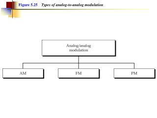
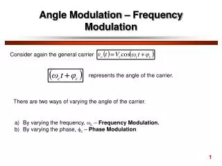
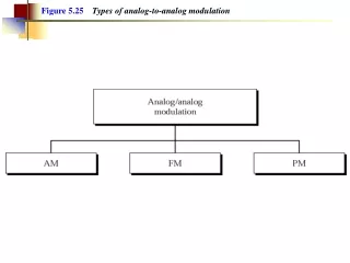
Impressing a message on the angle of carrier • There are two ways to form a an angle modulated signal. • Embed it in the phase of the carrier Phase Modulation(PM) • Embed it in the frequency of the carrier Frequency Modulation(FM) 1999 BG Mobasseri
Phase Modulation(PM) • In PM, carrier angle changes linearly with the message • Where • 2πfc=angle of unmodulated carrier • kp=phase sensitivity in radians/volt 1999 BG Mobasseri
Frequency Modulation • In FM, it is the instantaneous frequency that varies linearly with message amplitude, i.e. fi(t)=fc+kfm(t) 1999 BG Mobasseri
FM Signal • We saw that I.F. is the derivative of the phase • Therefore, 1999 BG Mobasseri
FM for Tone Signals • Consider a sinusoidal message • The instantaneous frequency corresponding to its FM version is 1999 BG Mobasseri
Illustrating FM Inst.frequency Moves with the Message amplitude 1999 BG Mobasseri
Frequency Deviation • Inst. frequency has upper and lower bounds given by 1999 BG Mobasseri
FM Modulation index • The equivalent of AM modulation index is which is also called deviation ratio. It quantifies how much carrier frequency swings relative to message bandwidth 1999 BG Mobasseri
Example:carrier swing • A 100 MHz FM carrier is modulated by an audio tone causing 20 KHz frequency deviation. Determine the carrier siwng and highest and lowest carrier frequencies 1999 BG Mobasseri
Example: deviation ratio • What is the modulation index (or deviation ratio) of an FM signal with carrier swing of 150 KHz when the modulating signal is 15 KHz? 1999 BG Mobasseri
Myth of FM • Deriving FM bandwidth is a lot more involved than AM • FM was initially thought to be a bandwidth efficient communication because it was thought that FM bandwidth is simply 2f • By keeping frequency deviation low, we can use arbitrary small bandwidth 1999 BG Mobasseri
FM bandwidth • Deriving FM bandwidth is a lot more involved than AM and it can barely be derived for sinusoidal message • There is a graphical way to illustrate FM bandwidth 1999 BG Mobasseri
Piece-wise approximation of baseband • Look at the following representation Baseband bandwidth =W 1/2W 1999 BG Mobasseri
Corresponding FM signal • FM version of the above is an RF pulse for each square pulse. • The frequency of the kth RF pulse at t=tk is given by the height of the pulse. i.e. 1999 BG Mobasseri
Range of frequencies? • We have a bunch of RF pulses each at a different frequency. • Inst.freq corresponding to square pulses lie in the following range mmax mmin 1999 BG Mobasseri
A look at the spectrum • We will have a series of RF pulses each at a different frequency. The collective spectrum is a bunch of sincs highest lowest f 4W 1999 BG Mobasseri
highest lowest f So what is the bandwidth? • Measure the width from the first upper zero crossing of the highest term to the first lower zero crossing of the lowest term 1999 BG Mobasseri
Closer look • The highest sinc is located at fc+kfmp • Each sinc is 1/2W wide. Therefore, their zero crossing point is always 2W above the center of the sinc. f 2W 1999 BG Mobasseri
highest lowest f Range of frequenices • Above range lies <fc-kfmp-2W,fc+kfmp+2W> 1999 BG Mobasseri
FM bandwidth • The range just defined is one expression for FM bandwidth. There are many more! BFM=4W+2kfmp • Using =∆f/W with ∆f=kfmp BFM=2(+2)W 1999 BG Mobasseri
Carson’s Rule • A popular expression for FM bandwidth is Carson’s rule. It is a bit smaller than what we just saw BFM=2(+1)W 1999 BG Mobasseri
Commercial FM • Commercial FM broadcasting uses the following parameters • Baseband;15KHz • Deviation ratio:5 • Peak freq. Deviation=75KHz BFM=2(+1)W=2x6x15=180KHz 1999 BG Mobasseri
Wideband vs. narrowband FM • NBFM is defined by the condition • ∆f<<W BFM=2W • This is just like AM. No advantage here • WBFM is defined by the condition • ∆f>>W BFM=2 ∆f • This is what we have for a true FM signal 1999 BG Mobasseri
Boundary between narrowband and wideband FM • This distinction is controlled by • If >1 --> WBFM • If <1-->NBFM • Needless to say there is no point for going with NBFM because the signal looks and sounds more like AM 1999 BG Mobasseri
Commercial FM spectrum • The FM landscape looks like this 25KHz guardband carrier FM station A FM station B FM station C 150 KHz 200 KHz 1999 BG Mobasseri
Left channel + mono + Right channel + FM stereo:multiplexing • First, two channels are created; (left+right) and (left-right) • Left+right is useable by monaural receivers - 1999 BG Mobasseri
Left channel + Composite baseband mono + + Right channel + DSB-SC fsc=38 kHz fsc= 38KHz freq divider Subcarrier modulation • The mono signal is left alone but the difference channel is amplitude modulated with a 38 KHz carrier - 1999 BG Mobasseri
Stereo signal • Composite baseband signal is then frequency modulated Composite baseband Left channel + FM transmitter mono + + Right channel + DSB-SC fsc=38 kHz - freq divider fsc= 38KHz 1999 BG Mobasseri
Left+right DSB-SC 19 KHz 38 KHz 15 KHz Stereo spectrum • Baseband spectrum holds all the information. It consists of composite baseband, pilot tone and DSB-SC spectrum 1999 BG Mobasseri
Left+right DSB-SC 19 KHz 38 KHz 15 KHz Stereo receiver • First, FM is stripped, i.e. demodulated • Second, composite baseband is lowpass filtered to recover the left+right and in parallel amplitude demodulated to recover the left-right signal 1999 BG Mobasseri
Receiver diagram + Left+right + left lowpass filter(15K) + coherent detector 15 KHz right - bandpass at 38KHz X lowpass + 19 KHz 38 KHz + FM receiver PLL X lowepass Divide 2 VCO 1999 BG Mobasseri
Subsidiary communication authorization(SCA) • It is possible to transmit “special programming” ,e.g. commercial-free music for banks, department stores etc. embedded in the regular FM programming • Such programming is frequency multiplexed on the FM signal with a 67 KHz carrier and 7.5 KHz deviation 1999 BG Mobasseri
SCA spectrum Left+right DSB-SC SCA signal 19 KHz 38 KHz 59.5 67 74.5 f(KHz) 15 KHz 1999 BG Mobasseri
FM receiver • FM receiver is similar to the superhet layout RF limiter Discrimi- nator mixer deemphasis IF LO AF power amp 1999 BG Mobasseri
Frequency demodulation • Remember that message in an FM signal is in the instantaneous frequency or equivalently derivative of carrier angle Do envelope detection on s’(t) 1999 BG Mobasseri
Receiver components:RF amplifier • AM may skip RF amp but FM requires it • FM receivers are called upon to work with weak signals (~1V or less as compared to 30 V for AM) • An RF section is needed to bring up the signal to at least 10 to 20 V before mixing 1999 BG Mobasseri
Limiter • A limiter is a circuit whose output is constant for all input amplitudes above a threshold • Limiter’s function in an FM receiver is to remove unwanted amplitude variations of the FM signal Limiter 1999 BG Mobasseri
Limiting and sensitivity • A limiter needs about 1V of signal, called quieting or threshold voltage, to begin limiting • When enough signal arrives at the receiver to start limiting action, the set quiets, i.e. background noise disappears • Sensitivity is the min. RF signal to produce a specified level of quieting, normally 1999 BG Mobasseri
Sensitivity example • An FM receiver provides a voltage gain of 200,000(106dB) prior to its limiter. The limiter’s quieting voltage is 200 mV. What is the receiver’s sensitivity? • What we are really asking is the required signal at RF’s input to produce 200 mV at the output 200 mV/200,000= 1V->sensitivity 1999 BG Mobasseri
Discriminator • The heart of FM is this relationship • What we need is a device that linearly follows inst. frequency fi(t)=fc+kfm(t) fcarrier is at the IF frequency Of 10.7 MHz Disc.output -75 KHz +75 KHz f fcarrier Deviation limits 1999 BG Mobasseri
output fc fo f Examples of discriminators • Slope detector - simple LC tank circuit operated at its most linear response curve This setup turns an FM signal into an AM 1999 BG Mobasseri
Phase-Locked Loop • PLL’s are increasingly used as FM demodulators and appear at IF output Output proportional to Difference between fin and fvco Phase comparator Lowpass filter fin Error signal Control signal:constant When fin=fvco VCO VCO input fvco 1999 BG Mobasseri
PLL states • Free-running • If the input and VCO frequency are too far apart, PLL free-runs • Capture • Once VCO closes in on the input frequency, PLL is said to be in the tracking or capture mode • Locked or tracking • Can stay locked over a wider range than was necessary for capture 1999 BG Mobasseri
PLL example • VCO free-runs at 10 MHZ. VCO does not change frequency until the input is within 50 KHZ. • In the tracking mode, VCO follows the input to ±200 KHz of 10 MHz before losing lock. What is the lock and capture range? • Capture range= 2x50KHz=100 KHz • Lock range=2x200 KHz=400 KHz 1999 BG Mobasseri