Download
1 / 15
150 likes | 266 Views
ECE 466/658: Performance Evaluation and Simulation. Introduction Instructor: Christos Panayiotou. Syllabus. Topics System Modeling and Modeling approaches Discrete Event Simulation Markov Chains Queueing Systems Queueing Networks Applications Additional Information

E N D
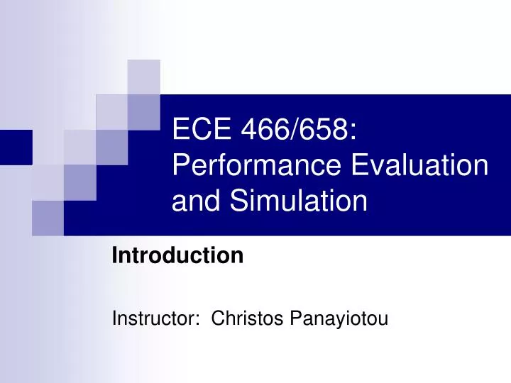
ECE 466/658: Performance Evaluation and Simulation Introduction Instructor: Christos Panayiotou
Syllabus • Topics • System Modeling and Modeling approaches • Discrete Event Simulation • Markov Chains • Queueing Systems • Queueing Networks • Applications • Additional Information • www.eng.ucy.ac.cy/christos/courses/ECE466 • www.eng.ucy.ac.cy/christos/courses/ECE658 • Topics have wide applicability… • Computer systems and networks • Manufacturing systems • Transportation systems • …
Need for Performance Evaluation • Computer system objectives • It must perform the functions that was designed for. • It must have adequate performance • Should perform its tasks under most circumstances • Should do them in reasonabletime and cost • When typing a text file, reasonable time is a few milliseconds whereas when running complicated simulations, reasonable may be a few days… • When designing a systems people usually pay a lot of attention to the functionality but not enough attention to the performance evaluation! • People address the issue of performance once the system is built when it is generally more difficult and more costly to achieve better performance.
Modeling and Performance Evaluation • Once a system is built, we may be able to use it to measure its performance • Opportunities to redesign and reengineer the system are lost or become a lot more costly! • When the system’s performance depends on some parameters, how can we figure out the best parameter settings? • Alternatively, one can build a model of the system, analyze it, and predict the performance of the actual system based on the model. • This approach is more flexible allowing for redesign and reengineering before investing in the final system.
Modeling • Model • It is a set of equations or a piece of software (simulator) that imitates the behavior of the real system. • There may be several models that can capture the behavior of a system. • Modeling is mostly an art and not an exact science. • Depending on the answers we are looking for, models can be very detailed and complex or they can be very simple.
Modeling Process OUTPUT INPUT SYSTEM OUTPUT INPUT MODEL u(t) y=g (u) • A model predicts what the system’s output would be given an input u(t). • A model is as good as its input: garbage in, garbage out!
Concept of State OUTPUT INPUT • Suppose that at a time instant t1, u(t1)=a and y(t1)=Y. Then, at time t2, u(t2)=a then what is y(t2)=?. • Example • Let x(t)=x(t-1)+u(t) • y(u(t))=u(t)+x(t)+5 • The state of a system at time t0 is the information required at t0 such that the output y(t), for all t≥t0, is uniquely determined from this information and from the input u(t), t≥t0. MODEL u(t) y(t) =g(u(t), t)
State Space Modeling • State equations: The set of equations required to specify the state x(t) for all t≥t0given x(t0) and the function u(t). • State Space X: The set of all possible values that the state can take. • Examples:
Sample Path x6 x(t) x(t) x5 x4 x3 x2 x1 t t • Evolution of the state over time Continuous State Discrete State
Example: Warehouse u1(t) u2(t) • System Input • System Dynamics
Example: Warehouse Sample Path • System Dynamics • System Input u1(t) t u2(t) t x(t) t
System Classification x(t) x(t) x(t) x(t) t t t t Continuous State –Continuous Time Discrete State –Continuous Time Continuous State –Discrete Time Discrete State –Discrete Time
Deterministic and Stochastic Systems • In many occasions the input functions u(t) are not known exactly but we can only characterize them through some probability distribution. • Signal noise at a mobile receiver • Arrival time of customers at a bank • … • If the input function is not known exactly, then the state cannot be determined exactly, but it constitutes a random variable • A system is stochastic if at least one of its output variables is a random variable. Otherwise the system is deterministic. • In general, the state of a stochastic system defines a random process.
Closing… • Depending on the type of system and/or the objectives of the analysis, one may be interested in various measures • Average number of customers in the system • Number of packets dropped in an interval [0,T]. • Average delay in a system • … • The most general tool for answering the above questions is computer simulation, however, simulation does not provide good understanding of the problem. • There are no general analytical tools that can address problems of some complexity with adequate accuracy, however, analytical tools can be used to gain a better understanding of the nature of the problem.
Closing (2)… • Simple vs “real” models • Simple models can be used to gain a better “understanding” • More complex models may be used to imitate real “real” scenarios • Accuracy vs Complexity • When modeling a system, it is important to always have in mind what questions the specific model will help you answer. • Changing the questions, may require changing the model! • Some questions may require accuracy. • Does the network meet the requirement of only 0.1% packet loss? • Some questions may not require much accuracy • Comparing two designs (ordinal optimization) • What does measure mean? • What does it mean “packet loss probability does not exceed 0.1”? • What does it mean “packet loss probability does not exceed 10-3”? • What does it mean “packet loss probability does not exceed 10-6”?