Download

1 / 58
600 likes | 941 Views
Simulation. Chapter Ten. 13.1 Overview of Simulation. When do we prefer to develop simulation model over an analytic model? When not all the underlying assumptions set for analytic model are valid. When mathematical complexity makes it hard to provide useful results.

E N D
Simulation Chapter Ten
13.1 Overview of Simulation • When do we prefer to develop simulation model over an analytic model? • When not all the underlying assumptions set for analytic model are valid. • When mathematical complexity makes it hard to provide useful results. • When “good” solutions (not necessarily optimal) are satisfactory. • A simulation develops a model to numerically evaluate a system over some time period. • By estimating characteristics of the system, the best alternative from a set of alternatives under consideration can be selected.
13.1 Overview of Simulation • Continuous simulation systems monitor the system each time a change in its state takes place. • Discrete simulation systems monitor changes in a state of a system at discrete points in time. • Simulation of most practical problems requires the use of a computer program.
13.1 Overview of Simulation • Approaches to developing a simulation model • Using add-ins to Excel such as @Risk or Crystal Ball • Using general purpose programming languages such as: FORTRAN, PL/1, Pascal, Basic. • Using simulation languages such as GPSS, SIMAN, SLAM. • Using a simulator software program. • Modeling and programming skills, as well as knowledge of statistics are required when implementing the simulation approach.
10.2 Monte Carlo Simulation • Monte Carlo simulation generates random events. • Random events in a simulation model are needed when the input data includes random variables. • To reflect the relative frequencies of the random variables, the random number mappingmethod is used.
JEWEL VENDING COMPANY – an example for the random mapping technique • Jewel Vending Company (JVC) installs and stocks vending machines. • Bill, the owner of JVC, considers the installation of a certain product (“Super Sucker” jaw breaker) in a vending machine located at a new supermarket.
JEWEL VENDING COMPANY – an example of the random mapping technique • Data • The vending machine holds 80 units of the product. • The machine should be filled when it becomes half empty. • Daily demand distribution is estimated from similar vending machine placements. • P(Daily demand = 0 jaw breakers) = 0.10 • P(Daily demand = 1 jaw breakers) = 0.15 • P(Daily demand = 2 jaw breakers) = 0.20 • P(Daily demand = 3 jaw breakers) = 0.30 • P(Daily demand = 4 jaw breakers) = 0.20 • P(Daily demand = 5 jaw breakers) = 0.05 Bill would like to estimate the expected number of days it takes for a filled machine to become half empty.
Solution • Expected time between refills • Is this the good value or only a good estimation ?
Random number mapping – The Probability function Approach Random number mappinguses the probability function to generate random demand. A number between 00 and 99 is selected randomly. The daily demand is determined by the mapping demonstrated below. 34 34 0.30 34 34 34 0.20 0.20 34 34 0.15 34 34 0.10 0.05 45-74 26-44 26-44 10-25 75-94 00-09 Demand 95-99 0 1 2 2 3 4 5
Random number mapping – The Cumulative Distribution Approach 1.00 1.00 0.95 0.75 The daily demand X isdetermined by the random number Y between0 and 1, such that X is thesmallest value for whichF(X) ³Y. F(1) = .25 < .34 F(2) = .45 > .34 0.45 Y = 0.34 0.34 0.25 0.10 0.00 2 0 1 2 3 4 5
Simulation of the JVC Problem • A random demand can be generated by hand (for small problems) from a table of pseudo random numbers. • Using Excel a random number can be generated by • The RAND() function • The random number generation option (Tools>Data Analysis)
45-74 26-44 10-25 75-94 00-09 95-99 3 Simulation of the JVC Problem • An illustration of generating a daily random demand. • Since we have two digit probabilities, we use the first two digits of each random number. 0 1 2 3 4 5
Simulation of the JVC Problem The simulation is repeated and stops once total demand reaches 40 or more. The number of “simulated” days required for the total demand to reach 40 or more is recorded.
Simulation Results and Hypothesis Tests • The purpose of performing the simulation runs is to find the average number of days required to sell 40 jaw breakers. • Each simulation run ends up with (possibly) a different number of days. • A hypothesis test is conducted to test whether or not m = 16. Null hypothesis H0 : m= 16 Alternative hypothesis HA : m¹ 16
Simulation Results and Hypothesis Tests • The test: • Define a (the significance level). • Let n be the number of replication runs. • Build the t-statisticThe t-statistic can be used if the random variable observed (number of day required for the total demand to be 40 or more) is normally distributed, while the standard deviation is unknown. • Reject H0 if t > ta/2 or t <- ta/2 (ta/2 has n-1 degrees of freedom.)
Sales < 40 Trials< Max JVC – A Flow Chart Flow charts help guide the simulation program Trials = 1 Max=…; sales = 0 S = 0; S2 = 0 Day = 0 Yes No Determine Daily demand (D) Record day S = S + day S2 = S2 + Day2 Sales = Sales + D Day = Day + 1 No End Yes Trials = Trials + 1 Sales = 0 Day = 0
JVC – Excel Spreadsheet =MAX(A5:A105) =IF(C5<40,A5+1,"") =IF(C5<40,B6+C5,"") =IF(C5<40,VLOOKUP(RAND(),$K$6:$L$11,2),"") VLOOKUP TABLE Enter this data Drag A5:C5 to A105:C105
= (18+14+16...+20) / 10 = 16.6 s2 =[(18-16.6)2+(14-16.6)2+...+(20-16.6)2] = 5.1556 t = (16.6 - 16) / [ 2.2706/ ] = 0.836 For a = 0.05 and n-1 = 9 degrees of freedom , t0.05/2 = 2.262. • After running 10 simulation replications on Excel, we have the following results. Number of days to sell 40 or more Jaw Breakers
JVC – Excel Spreadsheet =(E3-16)/E4 • The p-value =.2966… This value is quite high compared to any reasonable significance level. • Based on this data there is insufficient evidence to infer that the mean number of days differs from 16. =TDIST(ABS(H5),9,2)
Estimating the Average Number of Days Before a Refill is needed. • To obtain more reliable results more runs are made. • Summary of results Replications Average # of dayst value t(0.025) 10 16.60 0.836 2.262 50 17.04 3.337 1.96 100 16.66 2.996 1.96 500 16.39 3.889 1.96 2500 16.52 11.582 1.96 10000 16.46 20.785 1.96 The z value
Determining Confidence Intervals • What is our best estimate for m? • Confidence interval might help answer this question • When n <30, a (1-a)% confidence interval is • When , a (1-a)% confidence interval is n is the number of replications. • Example: n = 10000, 95% confidence interval is [16.42,16.50]
13.5 Simulation Modeling of Inventory Systems • Inventory simulation models are used when underlying assumptions needed for analytical solutions are not met. • Typical inputs into the simulation model are • Order cost • Holding cost • Lead time • Demand distribution Typical output is the average total cost for a given inventory policy
10.3 Simulation Modeling of Inventory Systems – continued • Frequently, the Fixed-Time Simulationapproach is appropriate for the modeling of inventory problems. • The system is monitored periodically. • The activities associated with demand, orders, and shipments are determined, and the system is updated accordingly. • Typical output is the average total cost for a given inventory policy.
Frequently, the Fixed-Time Simulation approach is appropriate for the modeling of inventory problems. • The system is monitored periodically. • The activity associated with demand, orders, and shipments is determined, and the system is updated.
ALLEN APPLIANCE COMPANY • Allen Appliance stocks and sells a certain bread maker. • Data • Unit cost is $260. • Annual holding cost rate is 26% • Orders are placed at the end of a week, and arrive at the beginning of a week. • Ordering cost is $45 per order. • Backorder cost is $5 per unit per week. • Backorder administrative cost is $2 per unit.
Distributions • The number of retailers that wish to purchase bread makers can be described by the Poisson distribution with l = 2. • The demand per customer is given by the following empirical distribution P(demand = 1) = 0.10 P(demand = 2) = 0.15 P(demand = 3) = 0.40 P(demand = 4) = 0.35 • The lead time has the following empirical distribution P(lead time = 1 weeks) = 0.2 P(lead time = 2 weeks) = 0.6 P(lead time = 3 weeks) = 0.2 What is the optimal inventory policy for Allen?
Inventory Systems • (R,M) : order point, order up to level when the inventory level reaches R, the firm orders enough to bring the stock to a level M when the orders arrives • (R,Q) : order point, order quantity the firm orders Q units the level of the stock reaches the inventory level R
Average weekly demand = 0.10(1)+0.15(2)+0.40(3)+0.35(4) = 3 units • Weekly holding cost = Ch=(annual holding cost)*Wholesale cost)/52 = (26%*$200/52) = $1 per unit per week • Average lead time for delivery = 0.2(1) + 0.6(2) + 0.2(3) = 2 weeks
P(0) = 0.350 000-134 P(1) = 0.271` 135-405 P(2) = 0.271406-676 P(3) = 0.180 P(4) = 0.090 P(5) = 0.036 P(6) = 0.012 P(7) = 0.003 P(8) = 0.001 P(9) = 0.001 l = 2; t = 1 week P(X = k) = (lt)k e-lt k! SOLUTION • Constructing random number mappings for: The number of retailers Who order in a week 0000-134 1135-405 2 406-676 3 677-856 4 857-946 5 947-982 6 983-994 7 995-997 8 998 9 999 Retailers’ demand 1 00-09 2 10-24 3 25-64 4 65-99 Lead time 1 week 0-1 2 weeks 2-7 3 weeks 8-9
There are several cases of inventory cost to consider: • There is inventory at the beginning and at the end of a week. Average inventory = (Initial inventory + Ending inventory) / 2 Weekly holding cost = Ch (Average inventory) • There are backordered units at the beginning and at the end of a week. Average backorder = (initial backorders + ending backorders) / 2 Weekly backorder cost = Cs(Average backorder) + p(additional backorders during the week)
There is inventory at the beginning, and backordered units at the end of a week. (Average inventory) = ( Proportion of time “in stock” )(Average inventory) (Average backorder) = (Proportion of time “out of stock”)(Average backorder) Holding cost and backorder costs are calculated as before.
Example : • Stock at the beginning of the week : 3 • Demand during the week : 8 • Number of backorders at the end of the week : 5 Assumption : • in-stock period : 3/8 of the week • out-of-stock period : 5/8 of the week Results Average inventory level=.375(1.5)+0.625(0)= .5625 units Holding cost for the week = .5625($1)=$.5625 Average backorder level=.375(0)+0.625(2.5)= 1.5625 units Backorder cost for the week=1.5625($5)+5($2) =$17.8125
Holding cost A1($1) Backorder cost AB($5) Beginning backorders Ending backorders Inventory Demand Backorders / Reordering Costs WK B1 R1 #A R2 D E1 A1 BB #B EB AB R3 LT HC BC AC RC TC 1 25 650 2 33 3 98 4 7 18 21.5 0 0 0 -- -- $21.5 0 0 0 $21.5 2 18 776 3 26 3 91 4 96 4 11 7 12.5 0 0 0 2 2 $12.5 0 0 $45 $57.5 p(#B) • Simulation of the (R,Q) system Average backorders Lead time Order cost $45 An order must be placed because ending inventory is less than the reorder point (=10) Initial inventory Initial inventory Ending inventory Ending inventory Random number Demand Average inventory Random number Number of orders
Holding cost A1($1) Backorder cost AB($5) Beginning backorders Ending backorders Inventory Demand Backorders / Reordering Costs WK B1 R1 #A R2 D E1 A1 BB #B EB AB R3 LT HC BC AC RC TC 3 7 617 2 48 3 0 82 4 7 0 3.5 0 0 0 1 $3.5 0 0 0 $3.5 4 0 880 4 27 3 96 4 46 3 20 2 12 0 0 12 12 6 0 0 30 24 0 $54 5 13 421 2 44 3 0 84 4 7 6 9.5 0 0 0 9 3 $9.5 0 0 $45 $54.5 p(#B) • Simulation of the (R,Q) System. Average backorders Lead time Order cost $45 (0+12)/2 $5(Average inventory) $2(Number of new backorders) Ending inventory Beginning inventory = ending inv. last week+ order received - backorders accumulated = 0 +25 -12 Initial inventory Initial inventory Random number Demand Random number Average inventory Number of orders Ending inventory
Results for ten simulated weeks • Average weekly cost for the (R,Q) policy is (21.50 + 57.50 + 3.50 + 54.00 + …) / 10 = $30.68 • Average weekly cost for the (R,M) policy is $27.90 • Based on ten weeks runs the (R,M) policy is preferred. • More runs are needed to substantiate this result.
10.4 Simulation of a Queuing System • In queuing systems time itself is a random variable.Therefore, we use the next event simulationapproach. • The simulated data are updated each time a new event takes place (not at a fixed time periods.) • The process interactive approach is used in this kind of simulation (all relevant processes related to an item as it moves through the system, are traced and recorded).
CAPITAL BANKAn example of queuing system simulation • Capital Bank is considering opening the bank on Saturdays morning from 9:00 a.m. • Management would like to determine the waiting time on Saturday morning based on the following data:
CAPITAL BANK • Data: • There are 5 teller positions of which only three will be staffed. • Ann Doss is the head teller, experienced, and fast. • Bill Lee and Carla Dominguez are associate tellers less experienced and slower.
CAPITAL BANK • Data: • Service time distributions:Ann’s Service Time DistributionBill and Carla’s Service Time Distribution Service TimeProbability Service TimeProbability.5 minutes .05 1 minute .05 1 .10 1.5 .15 1.5 .20 2 .20 2 .30 2.5 .30 2.5 .20 3 .103 .10 3.5 .103.5 .05 4 .054.5 .05
CAPITAL BANK • Data: • Customer inter-arrival time distributioninter-arrival timeProbability .5 Minutes .65 1 .15 1.5 .15 2 .05 • Service priority rule is first come first served • A simulation model is required to analyze the service .
CAPITAL BANK – Solution • Calculating expected values: • E(inter-arrival time) = .5(.65)+1(.15+1.5(.15)+2(.05) = .80 minutes [75 customers arrive per hour on the average, (60/.8=75)] • E(service time for Ann) = .5(.05)+1(.10)+…+3.5(.05) = 2 minutes [Ann can serve 60/2=30 customers per hour on the average] • E(Service time for Bill and Carla) = 1(.05)+1.5(.15)+…+4.5(.05) = 2.5 minutes [Bill and Carla can serve 60/2.5=24 customers per hour on the average].
CAPITAL BANK – Solution • To reach a steady state the bank needs to employ all the three tellers (30+2(24) = 78 > 75).
CAPITAL BANK – The Simulation logic • If no customer waits in line, an arriving customer seeks service by a free teller in the following order: Ann, Bill, Carla. • If all the tellers are busy the customer waits in line and takes then the next available teller. • The waiting time is the time a customer spends in line, and is calculated by [Time service begins] minus [Arrival Time]
1.5 3.5 CAPITAL – Simulation Demonstration 1.5 1.5 1.5 1.5 1.5 Bill 1.5 1.5 1.5 Ann 1.5 MappingInterarrival time 80 – 94 1.5 minutes MappingAnn’s Service time 35 – 64 2 minutes
3 5.5 1.5 3.5 CAPITAL – Simulation Demonstration Bill Ann MappingInterarrival time 80 – 94 1.5 minutes MappingBill’s Service time 40 – 69 2.5 minutes
3 3.5 CAPITAL – Simulation Demonstration Waiting time
Average inter-arrivaltime = .80 minutes. CAPITAL – 1000 Customer Simulation • To determine the other performance measures, we can use Little’s formulas: • Average number of customers in line Lq =(1/.80)(1.67) = 2.0875 customers • Average number of customers in the system = (1/.80)(3.993) = 4.99 customers. • This simulation estimates two performance measures: • Average waiting time in line (Wq) = 1.67 minutes • Average waiting time in the system W = 3.993 minutes
Mapping for Continuous Random Variables • Example • The Explicit inverse distribution method can be used to generate a random number X from the exponential distribution with m = 2 (i.e. service time is exponentially distributed, with an average of 2 customers per minute). • Randomly select a number from the uniform distribution between 0 and 1. The number selected is Y = .3338. • Solve the equation: X = F-1(Y) = – (1/m)ln(1 – Y) = –(1/2)ln(1-.3338) = .203 minutes.
=RAND() Drag to cell B13 =-LN(1-B4)/$B$1 Drag to cell C13 Mapping for Continuous Random Variables – Using Excel