Download
1 / 33
340 likes | 609 Views
An acoustic wave equation for pure P wave in 2D TTI media. Ge Zhan, Reynam C. Pestana and Paul L. Stoffa. Sept. 21, 2011 . Outline. Motivation Introduction Theory TTI coupled equations ( coupled P and SV wavefield ) TTI decoupled equations ( pure P and pure SV wavefield )

E N D
An acoustic wave equation for pure P wave in 2D TTI media GeZhan, Reynam C. Pestana and Paul L. Stoffa Sept. 21, 2011
Outline • Motivation • Introduction • Theory • TTI coupled equations (coupled P and SV wavefield) • TTI decoupled equations (pure P and pure SV wavefield) • Numerical implementation • Numerical Results • Impulse response result • Wedge model result • BP TTI model result • Conclusions
Outline • Motivation • Introduction • Theory • TTI coupled equations (coupled P and SV wavefield) • TTI decoupled equations (pure P and pure SV wavefield) • Numerical implementation • Numerical Results • Impulse response result • Wedge model result • BP TTI model result • Conclusions Vs0=0
Motivation • Why go TTI (Tilted Transversely Isotropy)? • Isotropic assumption is not always appropriate (this fact has been recognized in North Sea, Canadian Foothills and GOM). • Conventional isotropic/VTI methods result in low resolution and misplaced images of subsurface structures. • To obtain a significant improvement in image quality, clarity and positioning. • Pure P wave equation VS. TTI coupled equations • TTI coupled equations are not free of SV wave. • SV wave component leads to instability problem. • To model clean and stable P wave propagation. Model VTI RTM TTI RTM
Outline • Motivation • Introduction • Theory • TTI coupled equations (coupled P and SV wavefield) • TTI decoupled equations (pure P and pure SV wavefield) • Numerical implementation • Numerical Results • Impulse response result • Wedge model result • BP TTI model result • Conclusions Vs0=0
Introduction • Coupled equations (suffer from shear-wave artifacts, unstable) • 4th-order equation: Alkhalifah, 2000; • 2nd-order equations: Zhou et al., 2006; Du et al., 2008; Duveneck et al., 2008; Fletcher et al., 2008; Zhang and Zhang, 2008. • Coupled equations (combined with shear-wave removal) • Settingε=δaround source: Duveneck, 2008; • Model smoothing: Zhang and Zhang, 2010; Yoon et al., 2010 • Decoupled equations (free from shear-wave artifacts) • Muir-Dellinger approximation(Dellinger and Muir, 1985; Dellinger et al., 1993; later reinvented by Stopin, 2001) • Approximated VTI dispersion relation: Harlan, 1990&1995; Fowler, 2003; Etgen and Brandsberg-Dahl, 2009; Liu et al., 2009; Pestana et al., 2011
Outline • Motivation • Introduction • Theory • TTI coupled equations (coupled P and SV wavefield) • TTI decoupled equations (pure P and pure SV wavefield) • Numerical implementation • Numerical Results • Impulse response result • Wedge model result • BP TTI model result • Conclusions Vs0=0
TTI Coupled Equations • Start with the P-SV dispersion relation for TTImedia, set Vs0=0 along the symmetry axis (”pseudo-acoustic” approximation) • TTI Coupled Equations • (Zhou, 2006; Du et al., 2008; Fletcther et al., 2008; Zhang and Zhang, 2008) θ North Vertical Tilted Axis Φ Tilted Axis Vp0=3000 m/s, epsilon=0.24 delta=0.1, theta=45 degree
TTI Coupled Equations • Re-introduce non-zero Vs0 (Fletcher et al., 2009), • the above equations become • Vs0=Vp0/2 Vs0=0 Vp0=3000 m/s, epsilon=0.24 delta=0.1, theta=45 degree
Outline • Motivation • Introduction • Theory • TTI coupled equations (coupled P and SV wavefield) • TTI decoupled equations (pure P and pure SV wavefield) • Numerical implementation • Numerical Results • Impulse response result • Wedge model result • BP TTI model result • Conclusions Vs0=0
Square-root Approximation • Exact phase velocity expression for VTI media (Tsvankin, 1996) where _ _ expand the square root to 1st-order (Muir-Dellinger approximation)
VTI Decoupled Equations P wave and SV wave phase velocity for VTI media P wave and SV wave dispersion relations for VTI media
VTI Decoupled Equations P wave and SV wave dispersion relations for VTI media coupled P & SV pure-SV pure-P • Vp0=3000 m/s epsilon=0.24delta=0.1
TTI Decoupled Equations • Replace ( , , ) by (, , ), and • Dispersion relations for TTI media
TTI Decoupled Equations • P-wave and SV-wave equations in 2D time-wavenumber domain
Outline • Motivation • Introduction • Theory • TTI coupled equations (coupled P and SV wavefield) • TTI decoupled equations (pure P and pure SV wavefield) • Numerical implementation • Numerical Results • Impulse response result • Wedge model result • BP TTI model result • Conclusions Vs0=0
Numerical Implementation • Pseudospectralin space coupled with REMin time.
Outline • Motivation • Introduction • Theory • TTI coupled equations (coupled P and SV wavefield) • TTI decoupled equations (pure P and pure SV wavefield) • Numerical implementation • Numerical Results • Impulse response result • Wedge model result • BP TTI model result • Conclusions Vs0=0
2D Impulse Responses ( epsilon > delta ) Tilted Axis Vertical θ Coupled Equations Vp0=3000 m/s epsilon=0.24 delta=0.1 theta=45 degree Vs0≠0 Vs0=0 Vs0≠0 Vs0=0 Decoupled Equations pure-SV pure-P pure-SV pure-P
2D Impulse Responses ( epsilon < delta ) Coupled Equations NaN NaN Vp0=3000 m/s epsilon=0.1 delta=0.24 theta=45 degree Vs0≠0 Vs0=0 Vs0≠0 Vs0=0 Decoupled Equations pure-SV pure-P pure-SV pure-P
Outline • Motivation • Introduction • Theory • TTI coupled equations (coupled P and SV wavefield) • TTI decoupled equations (pure P and pure SV wavefield) • Numerical implementation • Numerical Results • Impulse response result • Wedge model result • BP TTI model result • Conclusions Vs0=0
Wedge Model (coutesy of Duveneck and Bakker, 2011) theta (degree) Vp(km/s) delta epsilon
Wavefield Snapshots ( t =1 s) Vs0=0 pure-P Vs0≠0
Wavefield Snapshots ( t =1.5 s) instability Vs0=0 pure-P Vs0≠0
Wavefield Snapshots ( t =4 s) unstable Vs0=0 stable unstable pure-P Vs0≠0
Outline • Motivation • Introduction • Theory • TTI coupled equations (coupled P and SV wavefield) • TTI decoupled equations (pure P and pure SV wavefield) • Numerical implementation • Numerical Results • Impulse response result • Wedge model result • BP TTI model result • Conclusions Vs0=0
BP TTI Model theta Vp delta epsilon
Wavefield Snapshots ( t=4 s) insitibility Vs0=0 Vs0≠0 pure-P
RTM Image Model VTI RTM VTI RTM TTI RTM TTI RTM
Outline • Motivation • Introduction • Theory • TTI coupled equations (coupled P and SV wavefield) • TTI decoupled equations (pure P and pure SV wavefield) • Numerical implementation • Numerical Results • Impulse response result • Wedge model result • BP TTI model result • Conclusions Vs0=0
Conclusions • TTI coupled and decoupled equations have long history with many contributors and derivations and methods of implementation. • We have shown that the numerical implementation using pseudospectralin space coupled with REM in time provides stable, near-analytically-accurate and numerical clean results. • Due to many FFTs (7 terms for 2D, 21 terms for 3D) per time step in the implementation, large clusters are needed for practical applications.
Acknowledgments • The authors wish to thank King Abdullah University of Science and Technology (KAUST) for providing research funding to this project. • We would like to thank BP for making the TTI model and dataset available. • We are also grateful to Faqi Liu, Hongbo Zhou, John Etgenand Paul Fowler for many useful suggestions on this work.
Thank you for your attention! Questions?