Download
1 / 17
170 likes | 294 Views
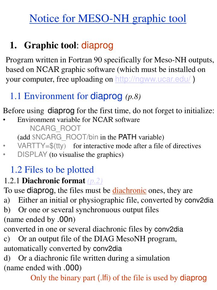
Notice for MESO-NH graphic tool. Graphic tool : diaprog. Program written in Fortran 90 specifically for Meso-NH outputs, based on NCAR graphic software (which must be installed on your computer, free uploading on http://ngww.ucar.edu/ ). 1.1 Environment for diaprog (p.8).

E N D
Notice for MESO-NH graphic tool • Graphic tool: diaprog Program written in Fortran 90 specifically for Meso-NH outputs, based on NCAR graphic software (which must be installed on your computer, free uploading on http://ngww.ucar.edu/ ) 1.1 Environment for diaprog(p.8) • Before usingdiaprog for the first time, do not forget to initialize: • Environment variable for NCAR software • NCARG_ROOT • (add $NCARG_ROOT/bin in the PATH variable) • VARTTY=$(tty) for interactive mode after a file of directives • DISPLAY (to visualise the graphics) 1.2 Files to be plotted • 1.2.1 Diachronic format(p.2) • To use diaprog, the files must be diachronic ones, they are • Either an initial or physiographic file, converted by conv2dia • Or one or several synchronuousoutput files • (name ended by .00n) • converted in one or several diachronic files by conv2dia • Or an output file of the DIAG MesoNH program, • automatically converted by conv2dia • Or a diachronic file written during a simulation • (name ended with .000) Only the binary part (.lfi) of the file is used by diaprog
Images are stored by diaprog in a file named gmeta (specific NCAR format) You have to rename it before use diaprog again. 1.2.2 Conversion of a synchronuous file by conv2dia File(s) to be converted must be splitted in .des and .lfi parts (otherwise use fm2deslfi to get .lfi or .Z.lfi ) conv2dia n file1 … filen filedia <- number of synchronuous files to convert <- name of the 1st synchronuous file <- name of the last synchronuous file <- name of the output diachronic file 1.3 ``Interactive’’ use of diaprog diaprog … … directives on keyboard … quit All the directives (keywords, precise syntax) are stored in an text file named dir.date:hh:mm to allow modifications and future use by diaprog< dir.date:hh:mm 1.4Graphic outputs To visualise images: idt gmeta To convert in PostScript: ctrans –d ps.color –q gmeta > gmeta.ps
The directives • taped on keyboard, or in a text file, • respect a strict syntax… • 80 characters maximum, character &, character ! • converted in upper case (except ‘filename’ and process name) • keywords between _ (ex: _PV_ ) 2.1 General directives (p.27) linvwb=tto invert black and white _file1_’filename’to open file (filename.lfi must be in DIRLFI directory) _file2_’otherfile’to open a 2nd file visuto open a graphic window lprint=tto get in a text file named FICVAL the values of the plotted fields lprintxy=tand the coordinate values convallij2ll to get the lat-lon values of all the grid points convij2xy=i1,,j1,i2,j2,9999. ‘’ of some grid points convxy2ij=lat1,lon1,9999.or vice versa 2.2 Directives to scan file(p.27) print groupsprint the ‘groups’ names of the current file print UM dim proc timeprint informations for the ‘group’ UM print filecurprint the name of current file opened print UM(i1:i2,j1:j2,k1:k2)print the values of the sub-array
2.3 Directives for plotting _file1_to select an opened file (if several opened) _T_to select a time (_T_time1 or _T_3600) _MINUS_(_PLUS_)difference or sum between 2 fields _ON_to superpose fields 2.3.1 Horizontal section (p.37) • Iso-surface (3D fields) p.42 _K_on a model level, ex: _K_20 _Z_on an altitude level (m), ex: _Z_5000 _PR_on an isobaric level (hPa), ex: _PR_850 (if PABSM or PABST in the file) _TK_on an isentropic level (K), ex: _TK_320 (if THM or THT in the file) _EV_on a potential vorticity level (PVU), ex: _EV_2 (if POVOM or POVOT in the file) _SV3_on any level (LXYZ00=T CGROUPSV3=‘gpe_nam’ ) • Section limits (p.44) default: the whole simulation domain (physical domain) or zoom with NIINF= NISUP= NJINF= NJSUP= • Horizontal wind (p.39) Name UM, VM (or UT, VT or UMnn, VMnn) Module: MUMVM Vectors: UMVM, stream lines: LSTREAM=T Direction: DIRUMVM 2.3.2 Horizontal profile (p.51) • // to the axes: NIINF=NISUP: //Y , NJINF=NJSUP: //X • Other orientation: intersection of a horizontal section and • vertical one ( _CV__K_,or_CV__Z_, or_CV__PR_, …)
2.3.3 Vertical section (p.60) _CV_ p.67 • defined by 4 different ways • NIDEBCOU= (or XIDEBCOU) NJDEBCOU= (or XJDEBCOU) NLANGLE= NLMAX= • LDEFCV2IND=T NIDEBCV= NJDEBCV= NIFINCV= NJFINCV= • LDEFCV2=T XIDEBCV= XJDEBCV= XIFINCV= XJFINCV= • LDEFCV2LL=T XIDEBCVLL=lat1 XJDEBCVLL=lon1 XIFINCVLL=lat2 XJFINCVLL=lon2 • vertical bounds • XHMIN= XHMAX= • or LPRESY=T XPMIN= XPMAX= XPINT= • LTRACECV=T(trace of the vertical section in a horizontal plan) • LCVZOOM=T(computation of isolines for the displayed zoom) • wind plotting • ULM (ULT)tangential component • VTM (VTT)transversal component • ULMWM (ULTWT)vectors p.70 • horizontal wind:MUMVM, UMVM, DIRUMVM 2.3.4 Vertical profile (p.73) _PV_ • defined by a vertical section and the localisation of the profile: • PROFILE= p.79 _PVT_ • temporal evolution of a profile with isolines p.81 _PVKT_ • temporal evolution of a profile with individual levels p.82 2.3.5 Radio-sounding (p.87) _RS__T_time1 or _RS1__T_time1 • definition: NIRS= NJRS= or XIRS= XJRS= p.90
2.3.6 Operations on fields(p.93) • Sum with a constant value, ex: THM(-273.15)_PR_850 • Multiplication by a constant value, ex: PABSM(*1e-2)_Z_500 • Multiplication (or division) of a field by another one • *expr1= (or /expr1=) 2.4 Presentation parameters of an image • Gestion of the plotting window (p.96) • Gestion of the axis • vertical bounds: according the type of plot • number of graduation of the axis (p.97) • format of the labels (p.98) • Gestion of the titles (p.99) • Gestion of the isolines (p.101) • NIMNMX= • Gestion of the arrays (p.116) • NISKIP= XVRL= • Gestion of the color (p.120) p.118 • LCOLINE=T • LCOLAREA=T Do not forget the documentation in html format on the web site: http://www.aero.obs-mip.fr/mesonh/index2.html Section ``Books and guides’’
Temporal evolution of a vertical profile (isolines)
Temporal evolution of a vertical profile (individual levels)