Download
1 / 19
190 likes | 275 Views
( e ,P) matrix. m. apollonio. 1. Gen e ral Introduction. the goal of MICE is demonstrating Ionisation Cooling … … for a variety of initial emittances momenta ideally covering a continuos space ( e ,P) practically studying some discrete points i.e. defining a matrix

E N D
(e,P) matrix m. apollonio CM26 - Riverside 1
General Introduction • the goal of MICE is demonstrating Ionisation Cooling … • … for a variety of initial • emittances • momenta • ideally covering a continuos space (e,P) • practically studying some discrete points • i.e. defining a matrix • the choice for it is: • eN = 3 / 6 / 10 mm rad • Pm= 140 / 200 / 240 MeV/c (at the centre of the H2 absorber) (*) 700mV ~ 20 mu-/spill CM26 - Riverside 2
P (MeV/c) • finding the element (3,240) means to find the BL optics that matches the MICE optics for a beam of 3 mm rad at a P=240 MeV/c 3,140 3,200 3,240 6,140 6,200 6,240 eN (mm rad) • the element (10,200) is the BL optics matching a MICE beam with 10 mm rad at P=200 MeV/c 10,140 10,200 10,240 This pair is our goal: how do we get it? CM26 - Riverside 3 (*) 700mV ~ 20 mu-/spill
Hyp.: eN0 is known (~1 mm rad trace space) • we proceed backward: • fix P/eN in the cooling channel • fix the optics in the cooling channel (a3,b3) • solve the equations giving a,b and t at the US face of the diffuser (*) b0 a0 Diffuser b1 a1 b2 a2 b3 a3 t BL MICE e1 (*) MICE note 176 e0 CM26 - Riverside 4
So the question becomes: • how do we “tell” the beamline to be a0, b0 at US_Diff? • solution(s) • we optimise the BL by varying Q4-Q9 • let us break the BL in two parts: US and DS • in what follows I mean a p m beamline Q1 Q2 Q3 Q4 Q5 Q6 Q7 Q8 Q9 Dipole1 Dipole2 DK solenoid • DS part: • choose Q4-Q9 • shoot a beam • check a,b at Diffuser vs “target” values • repeat m p • US part: we can optimise the MAX number of pions • but not much magic left … CM26 - Riverside 5
p m beam line: typical m spectrum at the exit of the DS • Rationale • select p u.s. of DKSol with D1 • select m d.s. of DKSol with D2 • back scattered muons == purity CM26 - Riverside
we already have an initial solution: the “central value” • Key Point • materials in the BL cause energy loss • (also emi_growth) • in order to have P_mice=200 MeV/c we need to define P_D2 properly • then we define Ppi_tgt • how? • the best choice is dictated by beam purity 3,140 3,200 3,240 6,140 6,200 6,240 10,140 10,200 10,240 CM26 - Riverside
m kinematic limits 445 MeV/c 350 MeV/c 250 MeV/c 195 MeV/c CM26 - Riverside
In the original scheme the pi mu beamline is Ppi=444 Pmu=256 Best separation PI/MU p acceptance Will it work? Pdiff = 215 NB.: PD2=256 MeV/c becomes Pdif=215 MeV/c CM26 - Riverside
3,140 Pdif=151 a=0.2 b=0.56m t=0.0mm 3,200 Pdif=207 a=0.1 b=0.36m t=0.0mm 3,240 Pdif=245 a=0.1 b=0.42m t=0.0mm 6,140 Pdif=148 a=0.3 b=1.13m t=5.0 6,200 Pdif=215 a=0.2 b=0.78m t=7.5mm 6,240 Pdif=256 a=0.2 b=0.8m t=7.5mm 10,140 Pdif=164 a=0.6 b=1.98m t=10mm?? 10,200 Pdif=229 a=0.4 b=1.31m t=15.5mm 10,240 Pdif=267 a=0.3 b=1.29m t=15.5mm CM26 - Riverside
i.o.t. accommodate several mu momenta another “shortcut” scheme was adopted (aug 2009): Define one lower Ppi ~ 350/360 and several different Pmu (we lose in purity …) p acceptance Pdiff = 148 215 256 Ppi (tgt) = 350 195 350 CM26 - Riverside
d.s. BL tuning: match to diffuser m Q1 Q2 Q3 Q4 Q5 Q6 Q7 Q8 Q9 Dipole1 Dipole2 DK solenoid p fix D2 fix D1 Pp=444 MeV/c Pm=255 MeV/c Pm=214 MeV/c Pm=208 MeV/c CM26 - Riverside 12
- a first round of the BL optimised • (e,P) matrix has been produced • in august 2009 (“shortcut”) • however the few data taken in november • reveal a pretty strange look • one thing I dislike is using only one • momentum for the pion (US) component and • Select the backward going muons CM26 - Riverside
http://mice.iit.edu/bl/MATRIX/index_mat.html CM26 - Riverside
~29. RUN 1174-1177 – PI- (444MeV/c) MU- (256 MeV/c) at D2 PI- should be here: 30.44 NB: DTmu(256)= DTmu(300) * beta300/beta256 = 28.55 * .943/.923 = 29.13 CM26 - Riverside
? PI- should be here: 30.44 RUN 1201 – PI- (336.8MeV/c) MU- (256 MeV/c) at D2 MU- should be the same as before … what is that? CM26 - Riverside
Generate Gaussian Beam with defined COV-MAT (arbitrary statistics) G4Beamline Generation up To DS x’ COV-MAT x y’ CM26 - Riverside y
wrap-up … • Consider all 9 cases: one Ppi + one Pmu per case (no “shortcuts”) • Define initial BL currents (from scaling tables) • Check tuning with G4Beamline • use simulation output at DS to infer the COV-MAT of the beam • Generate a Gauss-beam with that CovMat: • E.g. MatLab tool, fast + any number of particles … • Propagate / optimise this beam in the DS section • By hand (GUI tool) • By algorithm (GA) • check results versus real data … CM26 - Riverside