Download
1 / 44
450 likes | 585 Views
Ph.D. COURSE IN BIOSTATISTICS DAY 3. Example: Serum triglyceride measurements in cord blood from 282 babies (Data file: triglyceride.dta ). m = sample mean s = sample standard deviation. m-2s m-s m m+s m+2s. The distribution of serum triglyceride does not look like a normal

E N D
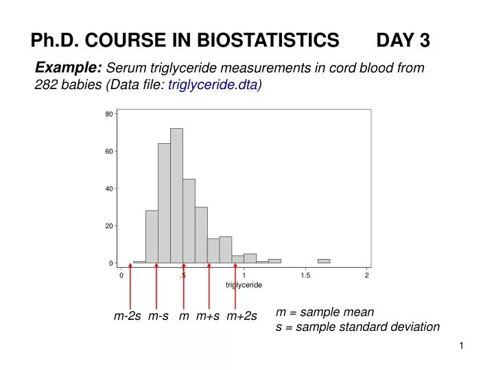
Ph.D. COURSE IN BIOSTATISTICS DAY 3 Example: Serum triglyceride measurements in cord blood from 282 babies (Data file: triglyceride.dta) m = sample mean s = sample standard deviation m-2s m-s m m+s m+2s
The distribution of serum triglyceride does not look like a normal distribution. The distribution is skew to the right or positively skew. A Q-Q plot clearlyshows the lack of fit. How should we summarize these data? How should we compare two groups of measurements for which the variation is positively skew?
Solution 1: A “non-parametric” approach Mean and standard deviations are mainly useful for symmetric distributions. For a skew distribution the “upward spread” differs from the “downward” spread, and a single number summary of the spread is therefore not sufficient. Summary statistics useful for skew distributions: median, 25, 75 percentiles or e.g. median, 5, 95 percentiles The skewness can be identified from these statistics. • tabstat trigly , stat(p5 med p95) variable | p5 p50 p95 -------------+------------------------------ trigly | .27 .46 .88 -------------------------------------------- Note: If a distribution is symmetric then mean = median If a distribution is skew to the right then mean > median. If a distribution is skew to the left then mean < median
Solution 2: Transformation of data A transformation of the data may lead to data that conform with a normal distribution. Statistical methods based for data from a normal distribution may then be applied to the transformed data. In principle many different transformations could be considered, but interpretation of results based on transformed data, may be complicated, so in practice only a few simple transformations e.g. the power transformations and in particular logarithm transformations, are used. Here we look at logarithm transformations: Data, original scale Data log-transformed Logarithms satisfy Natural logarithms are usually preferred for calculations. Figures with a logarithmic scale usually apply a logarithm to base 10. Basic facts about logarithms: see www.biostat.au.dk/teaching/praegrad/opgaver/biostat/logaritmefunktioner.pdf
On a log-scale pairs of points with the same ratio have the same distance, e.g. log(10) - log(5) = log(100) – log(50). Log-transformations therefore remove (or reduce) positive skewness. histogram trigly , /// xscale(log)start(0.1) width(0.1) freq log-scale with original units The figure suggests that on a log-scale the variation in the triglyceride data may be described by a normal distribution.
To obtain a more satisfactory histogram the log-transformed data must be generated explicitly natural logarithm can also be written as ln gene logtri=log(trigly) histogram logtri , freq start(-1.86) normal qnorm logtri , mco(blue) log-scale with natural log-units original units 0.14 0.38 1.00 On a log-scale these data look like a sample from a normal distribution, but can we interpret results derived from log-transformed data?
ANALYSIS OF LOG-TRANSFORMED DATA. INTERPRETATION OF RESULTS • On a log-scale the triglyceride data can be described by a normal • distribution, so on a log-scale the data are usefully summarized by • a mean and a standard deviation, • but what does these numbers mean? Consider a random variable X and introduce Z = log(X). The logarithm is here the natural logarithm, sometimes also called ln. Percentiles of the distribution of X are transformed to the analogous percentiles of the distribution of Z. In particular The exponential function exp is the inverse of the natural logarithm, so percentiles are easily “back-transformed, in particular
Similar results are not true for mean and standard deviation If the transformed variable Z follows a symmetric distribution we have so, when “back transformed” the sample mean of the log-transformed observations becomes an estimate of the median on the original scale, i.e. is an estimate of median(X). If the transformed variable follows a normal distribution further results are avialable:
If the transformed variable Z follows a normal distribution, the standard deviation of Z can be used to estimate c.v.(X), the coefficient of variation of X. The relations above show that The approximation is accurate if the variation is small, e.g. The coefficient of variation is often used to describe the variation of postively skew distributions. The result above shows that - unless the variation is large - the standard deviation of the log-transformed data, , can be used as an estimate of the coefficient of variation of the observations on the original scale. If the variation is large the coefficient of variation of X is estimated by
Confidence intervals Assume that the log-transformed data follow a normal distribution Confidence intervals for mean(Z) are ”back-transformed” to confidence intervals for median(X). Let and denote the lower and upper 95% confidence limits for then and are 95% confidence limits of the median(X). Similarly, by inserting the confidence limits for in the relation confidence limits for the coefficient of variation of X are obtained.
Two independent samples Consider two independent samples and . Assume that the sample distributions are positively skew, but that the log-transformed samples and can be described by normal distributions. The hypothesis of identical means on a log-scale corresponds to the hypothesis median(X) = median(Y). The ”back-transformed” difference is and estimate of the ratio Similarly, the confidence interval for transform back to a confidence interval for the ratio of the medians. The F-test of the hypothesis is equivalent to testing the hypothesis c.v.(X) = c.v.(Y).
Example – triglyceride data Summary statistics for skew data Solution 1 ( a non-parametric approach) • tabstat trigly , stat(p5 p25 p50 p75 p95) variable | p5 p25 p50 p75 p95 -------------+-------------------------------------------------- trigly | .27 .36 .46 .6 .88 ---------------------------------------------------------------- The population median is estimated by the sample median of 0.46. For later comparison we also compute the sample c.v. of X: • tabstat trigly , stat(mean sd cv) variable | mean sd cv -------------+------------------------------ trigly | .507153 .2184926 .4308218 -------------------------------------------- The population c.v. is estimated by the sample c.v. of 43%.
Example – triglyceride data Summary statistics for skew data Solution 2 ( log-transformation of data) tabstat logtri , stat(p5 p25 p50 p75 p95) variable | p5 p25 p50 p75 p95 -------------+-------------------------------------------------- logtri | -1.309333 -1.021651 -.7765288 -.5108256 -.1278334 ---------------------------------------------------------------- Percentiles transform back to percentiles, e.g. exp(-1.309333) = 0.27 and exp(-0.7765288) = 0.46 Confidence interval for the median of X tabstat logtri , stat(mean semean sd var) variable | mean se(mean) sd variance -------------+---------------------------------------- logtri | -.7570465 .0231264 .3876687 .1502871 ------------------------------------------------------ We compute a confidence interval for mean(Z) and transform the limits back to the original scale.
lower limit: upper limit: 95% confidence limits for median(X) therefore become exp(-0.8026) = 0.45 and exp(-0.7115) = 0.49. We can also compute a 90% prediction interval based a normal distribution for Z and transform back to the original scale. as expected these values are very similar to the 5 and 95 percentiles. Estimation of c.v.(X): The standard deviation is here a rather crude estimate of c.v.(X), instead we use The estimate is very similar to the estimate computed from the sample mean and the sample standard deviation of the original data.
Why use transformations of data? Why ”change the data to fit the method”? – instead of ”change the method to fit the data”? For simple problems a simple solution is OK: Use sample percentiles as descriptive statistics and non-parametric tests for statistical inference. Transformation of data • For more complicated problems the methods available assume that • data are from a normal population. The choice is then between • A simple, but unsatisfactory analysis • An satisfactory analysis based on transformed data. The methods based on a normal distribution are appealing because they are more powerful and cover a wider range of problems. Disadvantages: Interpretation and presentation of results from analyses of transformed data is not always straightforward.
THE TWO-SAMPLE PROBLEM WITH PAIRED DATA Example:Measurement of body temperature The Stata file temp.dta contains measurements of body temperature in 96 patients using Rectal Hg thermometer, Oral Hg thermometer, and an electronic device (Craft-thermometer). • list id hgrectal hgoral craft in 1/5 +--------------------------------+ | id hgrectal hgoral craft | |--------------------------------| 1. | 1 38.1 37.1 37.4 | 2. | 2 38.1 37.8 37.8 | 3. | 3 38.9 38.2 38.2 | 4. | 4 38.4 38.2 38.1 | 5. | 5 40.3 40 40.1 | +--------------------------------+ The data were collected as part of a study to assess the validity of the electronic thermometer. Here we consider the two series of HG thermometer readings.
A plot of 94 pairs of readings of oral and rectal Hg temperatur (two patients had missing rectal reading) identity line
Questions: • What is the difference between oral and rectal body temperature? • How much does the differences vary between patient? The situation resembles the two-sample problem discussed in lecture 2, but here the same patients are measured with both methods. We no longer have two independent samples, but two paired samples. • The “obvious” analysis • For each patient compute the difference between the two readings • Provided the assumptions are satisfied the differences are modeled as • a sample for from a normal distribution: compute a confidence intervals • for the expected difference and the standard deviation and perhaps a • one-sample t-test of the hypothesis that the expected difference is 0. If the normal distribution does not apply, use a non-parametric approach instead (Lecture 5).
Note: • The obvious approach was used for the analysis of the data on • change in diastolic blood pressure (Lecture 2). • The data may be used to identify systematic differences between • the methods (accuracy), but replicate measurements are needed • to describe the random measurement error (precision). What kind of model considerations leads to this analysis? • Consider a given patient and introduce the following notation • X = A reading of the rectal Hg temperature • Y = A reading of the oral Hg temperature • and let • D = X – Y = the difference between the two readings. • The temperature readings X and Y can be considered as a sum of • two components: • X = A + E • Y = B + F
Here • A = the “true” rectal temperature, i.e. the hypothetical value we • would obtain as the average reading if the “experiment” was • repeated a large number of times • B = the “true” oral temperature • E = the random measurement error associated with a • rectal temperature reading using a Hg thermometer • F = the random measurement error associated with an • oral temperature reading using a Hg thermometer • The difference D is therefore • D = (A – B) + (E – F) • The first term, A – B, represents the difference between true rectal and • oral temperature for the given patient on a given day. • The second term, E – F, is the combined effect of measurement errors.
In a population of patients the difference of true temperatures, A – B, • may vary between individuals and also between days for a given • individual. Let denote the population mean, then • A – B = + C, • where C represents intra-individual variation in difference • in true temperature. • Returning to the difference between the readings we therefore have the • following decomposition • D = X – Y = + (C + E – F) = + U, • where is the population mean and U decribes random variation, • which has three components, inter-individual variation in true differences, • measurement error of rectal reading, measurement error of oral reading. The statistical model underlying the ”obvious” approach describes the data as a random sample from a normal distribution with mean and variance .
Note: The model describes the differences and does not specify anything about the variation of temperature (rectal or oral) in the population of patients (A or B is not assumed to vary according to a normal distribution). • Checking the validity of the assumptions: • Independence: Reasonable here, since each patient contributes with one difference only. • Same distribution: • The expected difference between the two readings does not depend on the overall level of the temperature. Is this a reasonable assumption? • The random variation in the difference has the same size for all temperatures. Is this a reasonable assumption? • Normal distribution:Is this a reasonable assumption?
Important plots that should always be made: • A plot of Y against X • Difference against average (or against sum) • Histogram of differences • Q-Q plot of differences a b c d
The plots were made using a Stata do-file with the following commands scatter hgoral hgrectal , /// title("Oral Hg versus Rectal Hg") /// ylabel(35(1)41) xlabel(35(1)41) /// saving(g1, replace) mco(gs3) gene difro = hgrectal-hgoral gene hgmean=(hgrectal+hgoral)/2 scatter difro hgmean , /// title("difference versus average") /// ylabel(-0.8(0.4)1.6) xlabel(37(1)41) /// saving(g2,replace) mco(gs3) histogram difro , /// title("Rectal Hg - Oral Hg") /// start(-0.8) width(0.2) /// saving(g3,replace) qnorm difro , title("Q-Q plot of difference") /// saving(g4,replace) mco(gs3) graph combine g1.gph g2.gph g3.gph g4.gph , /// saving(g5,replace)
Plot a: Oral reading versus rectal reading Comments No systematic differences are present if the points would scatter around the identity line (red line). The plot suggests that rectal temperature is systematically higher, but the size of the difference does not seem to vary systematically over the range of temperatures. The points scatter around a line with slope 1 (black line) is fairly constant over the range of temperatures.
Plot b: Difference versus average. Often called a Bland- Altman plot Comments If no systematic differences are present the points scatter around the horizontal line at 0 (red line). The plot suggests that rectal temperature is systematically higher, but the size of the difference does not seem to vary systematically over the range of temperatures. The points scatter around a horizontal line at approx. 0.5 (black line) and the variation is fairly constant over the range of temperatures.
Plot c and d: The histogram and the Q-Q plot of the difference. Comments: These plots are mainly used for assessing the validity of a normal distribution. The distribution looks fairly symmetric with a modest departure from the normal curve. The slightly S-shaped pattern in the Q-Q plot indicates that both tails are too long. This could be the consequence of a few gross errors.
Analysis using Stata: • A paired two-sample problem can be analyzed with the command • ttest directly, i.e. without first generating the difference • ttest hgrectal=hgoral == is also allowed Paired t test --------------------------------------------------------------------- Variable | Obs Mean Std. Err. Std. Dev. [95% Conf. Interval] ---------+----------------------------------------------------------- hgrectal | 94 38.06808 .0852441 .8264723 37.89881 38.23736 hgoral | 94 37.57447 .0855485 .8294235 37.40459 37.74435 ---------+----------------------------------------------------------- diff | 94 .4936168 .0330279 .3202179 .4280298 .5592038 --------------------------------------------------------------------- mean(diff) = mean(hgrectal - hgoral) t = 14.9454 Ho: mean(diff) = 0 degrees of freedom = 93 Ha: mean(diff) < 0 Ha: mean(diff) != 0 Ha: mean(diff) > 0 Pr(T < t) = 1.0000 Pr(|T| > |t|) = 0.0000 Pr(T > t) = 0.0000 average difference 95% confidence limits for the expected difference p-value of the hypothesis that the expected difference is 0
Analysis, continued Estimates obtained form the output 95% confidence limits for becomes (see Lecture 2 page 31): Conclusion: Rectal Hg temperature is on the average 0.5 degree higher than oral Hg temperature. The random variation (measurement errors and inter- and intra-individual variation) has a standard deviation of 0.32 degree. The confidence interval of the expected difference does not describe the agreement between the two methods. Limits of agreement are defined as (i.e. mean diff. ± 2·s.d.). This is an approx. 95% prediction interval. The limits are rather wide: -0.15 and 1.13 reflecting the relatively large variation in the differences.
Example Urinary albumin excretion rate The file albu.dta contains data on urinary albumin excretion rate (µg/min) measured by two different methods (“one-hour” and “night”) in 15 patients. Diagnostic plots a. b. d. c.
Example T4 and T8 cell concentration The file tcounts.dta contains data on the number of T4 and T8cell/mm3 in blood samples from 20 patients in remission from Hodgkin’s disease. Diagnostic plots a. b. d. c.
In both of these examples the difference between the two values increases with the size. Also the variation in the difference seems to increase with the size of the measurements. The ”obvious” analysis may not be apppropriate, but do we have any alternatives?
PAIRED DATA: ABSOLUTE OR RELATIVE CHANGE/DIFFERENCE? • Data: a sample of size n of pairs of observations (x,y). • Such data arise in many situations, e.g. • Comparison of measurement methods • Comparison of pre-treatment and post-treatment measurements • Studies of inter-observer or intra-observer variation Problem: Do the x’s differ from the y’s? If yes, how? First reaction: Look at differences (the obvious analysis above) BUT should we consider absolute or relative difference/change? Absolute change Relative change note: the relative change is just the ratio ”adjusted” such that 0 becomes the ”no change” value.
Absolute or relative change? The choice should reflect the structure of the systematic variation in the data. • The relationship between the two series of measurements may identify • the most appropriate choice. • Two simple relations between y and x • 1. • 2. In situation 1 differences will be relatively stable. If the variation in the data conforms to this relation absolute change is the appropriate choice (from a statistical perspective). In situation 2 ratios will be relatively stable. If the variation in the data conforms to this relation relative change is the appropriate choice (from a statistical perspective).
The paired t-test and the non-parametric analog are primarily intended for situation 1, since these tests are based on the differences. Situation 2 is often best handled by taking logarithms: i.e. the relationship between log(x) and log(y) is additive (situation 1) with a = log(b) In short: If the variation in a series of pairs (x,y) is multiplicative (situation 2) the best approach is usually to compute the differences and base the statistical analyses on these differences. This corresponds to working with ratios on a log-scale.
Paired data: Difference of logs versus relative change Why not use relative change in situation 2? Example • The second person is just a ”reversed version” of the first person, so • ”nothing happens”. • The first average (x) is identical to the second average (y). • The average relative change is 25% indicating a slight increase. • The average ratio is larger than 1 indicating a slight increase. • The average of difference of logs – the ratio measured on a log-scale – • is 0, indicating the sensible result: no change.
Paired data: Difference of logs versus relative change Working with ratios on a log-scale is convenient, since e.g. The relative change does not have this property When the ratio y/x is close to 1 then When the ratio is close to 1 (e.g. within ±20%) then the difference between the natural logarithms is approximately equal to the relative change. Paired data with a multiplicative structure (situation 2) usually also have an increased variability for large observations. Working with data on log-scale stabilize variation and may therefore lead to a simpler description of the random variation (a coefficient of variation).
Example T4 and T8 cell concentration The diagnostic plots (page 31) indicated that an additive relationship was inappropriate. Data are now log-transformed to evaluate the fit of a multiplicative structure. Diagnostic plots based on log-transformed data a. b. d. c.
Example T4 and T8 cell concentration – continued log-transformed data: Both systematic and random variation agree better with assumptions . • Stata analysis of log-transformed data • gene logt4=log(t4) • gene logt8=log(t8) • ttest logt4=logt8 Paired t test --------------------------------------------------------------------- Variable| Obs Mean Std. Err. Std. Dev. [95% Conf. Interval] --------+------------------------------------------------------------ logt4 | 20 6.486932 .1583811 .7083018 6.155437 6.818427 logt8 | 20 6.237297 .1371353 .6132875 5.95027 6.524325 --------+------------------------------------------------------------ diff | 20 .2496345 .1271238 .5685149 -.0164387 .5157076 --------------------------------------------------------------------- mean(diff) = mean(logt4 - logt8) t = 1.9637 Ho: mean(diff) = 0 degrees of freedom = 19 Ha: mean(diff) < 0 Ha: mean(diff) != 0 Ha: mean(diff) > 0 Pr(T < t) = 0.9678 Pr(|T| > |t|) = 0.0644 Pr(T > t) = 0.0322
ANALYSIS OF LOG-TRANSFORMED, PAIRED SAMPLES INTERPRETATION OF RESULTS Summary statistics in output describe , i.e. the ratio of the counts on a log-scale. The log-transformed ratios are a sample from a normal distribution. The relationships on page 7-10 show how to translate the results to results about the ratios. We have Ratio: Log scale Ratio: Original scale mean = 0.250 median = exp(0.250) = 1.28 conf.limits of mean conf. limits of median -0.016 0.516 0.98 1.67 standard deviation coefficient of variation 0.569 62% approx. 95% prediction interval approx. 95% prediction interval -0.89 1.39 0.41 4.00
The estimates above may be compared with estimates based on the • sample of ratios. • gene ratio=t4/t8 • tabstat ratio , stat(med cv min max) Note: the sample size is 20, so the ”non-parametric” 95% prediction limits are min and max Output variable | p50 cv min max -------------+---------------------------------------- ratio | 1.193993 .6085281 .4736842 3.818452 ------------------------------------------------------ The two sets of estimates agree reasonably well. Note: Usinglog-transformation in the analysis of two paired samples leads to an estimate of the median ratio. Using log-transformation in the analysis of two independent samples leads to an estimate of the ratio of the medians.
WHY USE TRANSFORMATION ÒF DATA? Overall purpose log transformation – and other transformations - of the data are often used because a simpler description of the transformed data is available. • Two aspects • Simpler description of the random variation: • A positively skew distribution was replaced by a symmetric distribution • Bland-Altman plot: on a log scale the size of variation was independent • of the level of the outcome • A simpler, and more valid, description of the systematic variation • For paired data the multiplicative structure was replaced by a • additive structure More advanced statistical methodology for continuous variables , e.g. regression models and analysis of variance models, assumes constant standard deviation and additivity of effects. Transformation of data may therefore be necessary to apply these methods.
Note: Whether or not to use t-test is often believed to be the most important question in analysis of two-sample problems. BUT the choice of appropriate measure of change is usually much more important than the choice of test statistic. Always look at diagnostic plots! However, sometimes there is no clear answer, because 1. Neither the original scale or a log-scale is appropriate • If the variation between pairs is modest it can be very difficult to • distinguish between an additive structure and a multiplicative • structure in the data. In such situations the results are usually very • similar for transformed and untransformed data. 3. The transformation that achieves additivity is not the transformation that achieves constant variation. 4. It is just a mess
STATA – some interactive commands Both ttest and sdtest have interactive versions, called ttesti and sdtesti, respectively. These commands do not require the full data set, but the relevant summary statistics are instead entered directly after the command. Some examples • one-sample problem: n = 213, mean = 1.901, sd = 7.529, H: mean = 0 • ttesti 213 1.901 7.529 0 • two-sample problem: n1 = 213, mean1 = 1.901, sd1 = 7.529, • n2 = 217, mean2 = 2.194, sd2 = 8.365 • H: mean1 = mean2 • ttesti 213 1.901 7.529 217 2.194 8.365 means are not necessary, write a period. • one-sample problem: n = 213, sd = 7.529, H: sd = 7 • sdtesti 213 . 7.529 7 • two-sample problem: n1 = 213, sd1 = 7.529, n2 = 217, sd2 = 8.365 • H: sd1 = sd2 • sdtesti 213 . 7.529 217 . 8.365