Download
1 / 109
1.13k likes | 1.3k Views
Single Area OSPF. (CCNA 3). Notes. Configuration of OSPF is easy. The concepts and theory that make it a robust and scalable protocol is a little more complex. Information in this presentation that goes beyond that which is presented in the CCNP 3.0 curriculum.

E N D
Single Area OSPF (CCNA 3)
Notes • Configuration of OSPF is easy. • The concepts and theory that make it a robust and scalable protocol is a little more complex. • Information in this presentation that goes beyond that which is presented in the CCNP 3.0 curriculum. • This information is included to give you a better understanding of OSPF, to answer some of the students’ questions, and to get an idea of the true operational features of OSPF. Routing TCP/IP Volume I by Jeff Doyle OSPF, Anatomy of an Internet Routing Protocol by John Moy (creator of OSPF) Rick Graziani graziani@cabrillo.edu
Preview of the OSPF Commands Required Commands: Rtr(config)# router ospf process-id Rtr(config-router)#network addresswildcard-mask area area-id Rick Graziani graziani@cabrillo.edu
Preview of the OSPF Commands Optional Commands: Rtr(config-router)# default-information originate (Send default) Rtr(config-router)# area area authentication (Plain authen.) Rtr(config-router)# area area authentication message-digest (md5 authen.) Rtr(config)# interface loopback number (Configure lo as RtrID) Rtr(config)# interface type slot/port Rtr(config-if)# ip ospf priority <0-255> (DR/BDR election) Rtr(config-if)# bandwidth kbps(Modify default bandwdth) RTB(config-if)# ip ospf cost cost (Modify inter. cost) Rtr(config-if)# ip ospf hello-interval seconds (Modify Hello) Rtr(config-if)# ip ospf dead-interval seconds (Modify Dead) Rtr(config-if)# ip ospf authentication-key passwd (Plain/md5authen) Rtr(config-if)# ip ospf message-digest-key key-id md5 password Rick Graziani graziani@cabrillo.edu
Introduction to OSPF Concepts Introducing OSPF and Link State Concepts • Advantages of OSPF • Brief History • Terminology • Link State Concepts Introducing the OSPF Routing Protocol • Metric based on Cost (Bandwidth) • Hello Protocol • Steps to OSPF Operation • DR/BDR • OSPF Network Types Rick Graziani graziani@cabrillo.edu
Advantages of OSPF (1 of 2) • OSPF is link-state routing protocol • RIP, IGRP and EIGRP are distance-vector (routing by rumor) routing protocols, susceptible to routing loops, split-horizon, and other issues. • OSPF has fast convergence • RIP and IGRP hold-down timers can cause slow convergence. • OSPF supports VLSM and CIDR • RIPv1 and IGRP do not Rick Graziani graziani@cabrillo.edu
Advantages of OSPF (2 of 2) • Cisco’s OSPF metric is based on bandwidth • RIP is based on hop count • IGRP/EIGRP bandwidth, delay, reliability, load • OSPF only sends out changes when they occur. • RIP sends entire routing table every 30 seconds, IGRP every 90 seconds • Extra: With OSPF, a router does flood its own LSAs when it age reaches 30 minutes (later) • OSPF also uses the concept of areas to implement hierarchical routing known as Multiarea OSPF Rick Graziani graziani@cabrillo.edu
Brief History • The first link-state routing protocol was implemented and deployed in the ARPANET (Advanced Research Project Agency Network), the predecessor to later link-state routing protocols. • Next, DEC (Digital Equipment Corporation) proposed and designed a link-state routing protocol for ISO’s OSI networks, IS-IS (Intermediate System-to-Intermediate System). • Later, IS-IS was extended by the IETF to carry IP routing information. • IETF working group designed a routing protocol specifically for IP routing, OSPF (Open Shortest Path First). • OSPF version 2, current version, RFC 2328, John Moy • Uses the Dijkstra algorithm to calculate a SPT (Shortest Path Tree) • Two open-standard routing protocols to choose from: • RIP, simple but very limited, or • OSPF and IS-IS, robust but more sophisticated to implement. • (IGRP and EIGRP are Cisco proprietary) Rick Graziani graziani@cabrillo.edu
Terminology • Link: Interface on a router • Link state: Description of an interface and of its relationship to its neighboring routers, including: • IP address/mask of the interface, • The type of network it is connected to • The routers connected to that network • The metric (cost) of that link • The collection of all the link-states would form a link-state database. Rick Graziani graziani@cabrillo.edu
Terminology • Router ID – Used to identify the routers in the OSPF network • IP address configured with the OSPF router-id command • Highest loopback address (configuration coming) • Highest active IP address(any IP address) • Loopback address has the advantage of never going down, thus diminishing the possibility of having to re-establish adjacencies. (more in a moment) Rick Graziani graziani@cabrillo.edu
Terminology CCNA 3.0 covers Single Area OSPF as opposed to Multi-Area OSPF • All routers will be configured in a single area, the convention is to use area 0 • If OSPF has more than one area, it must have an area 0 • CCNP includes Multi-Area OSPF • We will include a brief introduction to Multi-Area OSPF so you can see the real advantages to using OSPF Single Area OSPF uses only one area, usually Area 0 Or “OSPF Routing Domain” Rick Graziani graziani@cabrillo.edu
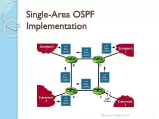
Link State Analogy • Link State Information: • Using separate index cards, write the your name and the student sitting next to you (including the student on your left, right, in front, in back). • Link State Flooding: • Pass all of the index cards to me (instructor) • Link State Database • This is the stack of index cards. • Typically we would all be working with the identical stack of cards. • SPF Algorithm • Using the cards I will map out who is sitting next to who for the entire class. • Routing Table Update • Now that I have a map of the class I can determine the best path to each student. Rick Graziani graziani@cabrillo.edu
Link State 1 – Flooding of link-state information 1 – Flooding of link-state information • The first thing that happens is that each node, router, on the network announces its own piece of link-state information to other all other routers on the network. This includes who their neighboring routers are and the cost of the link between them. • Example: “Hi, I’m RouterA, and I can reach RouterB via a T1 link and I can reach RouterC via an Ethernet link.” • Each router sends these announcements to all of the routers in the network. Rick Graziani graziani@cabrillo.edu
Link State 1 – Flooding of link-state information 2. Building a Topological Database • Each router collects all of this link-state information from other routers and puts it into a topological database. 3. Shortest-Path First (SPF), Dijkstra’s Algorithm • Using this information, the routers can recreate a topology graph of the network. • Believe it or not, this is actually a very simple algorithm and I highly suggest you look at it some time, or even better, take a class on algorithms. (Radia Perlman’s book, Interconnections, has a very nice example of how to build this graph – she is one of the contributors to the SPF and Spanning-Tree algorithms.) 3 – SPF Algorithm 2 – Building a Topological Database Rick Graziani graziani@cabrillo.edu
Link State 1 – Flooding of link-state information 4. Shortest Path First Tree • This algorithm creates an SPF tree, with the router making itself the root of the tree and the other routers and links to those routers, the various branches. 5. Routing Table • Using this information, the router creates a routing table. 5 – Routing Table 3 – SPF Algorithm 2 – Building a Topological Database 4 – SPF Tree Rick Graziani graziani@cabrillo.edu
Link State Concepts • How does the SPF algorithm create an SPF Tree? • Let’s take a look! • This is extra Information. 1 – Flooding of link-state information 5 – Routing Table 3 – SPF Algorithm 2 – Building a Topological Database 4 – SPF Tree Rick Graziani graziani@cabrillo.edu
Extra: Simplified Link State Example • In order to keep it simple, we will take some liberties with the actual process and algorithm, but you will get the basic idea! • You are RouterA and you have exchanged “Hellos” with: • RouterB on your network 11.0.0.0/8 with a cost of 15, • RouterC on your network 12.0.0.0/8 with a cost of 2 • RouterD on your network 13.0.0.0/8 with a cost of 5 • Have a “leaf” network 10.0.0.0/8 with a cost of 2 • This is your link-state information, which you will flood to all other routers. • All other routers will also flood their link state information. (OSPF: only within the area) 11.0.0.0/8 “Leaf” 10.0.0.0/8 12.0.0.0/8 2 13.0.0.0/8 Rick Graziani graziani@cabrillo.edu
Extra: Simplified Link State Example RouterB: • Connected to RouterA on network 11.0.0.0/8, cost of 15 • Connected to RouterE on network 15.0.0.0/8, cost of 2 • Has a “leaf” network 14.0.0.0/8, cost of 15 RouterC: • Connected to RouterA on network 12.0.0.0/8, cost of 2 • Connected to RouterD on network 16.0.0.0/8, cost of 2 • Has a “leaf” network 17.0.0.0/8, cost of 2 RouterD: • Connected to RouterA on network 13.0.0.0/8, cost of 5 • Connected to RouterC on network 16.0.0.0/8, cost of 2 • Connected to RouterE on network 18.0.0.0/8, cost of 2 • Has a “leaf” network 19.0.0.0/8, cost of 2 RouterE: • Connected to RouterB on network 15.0.0.0/8, cost of 2 • Connected to RouterD on network 18.0.0.0/8, cost of 10 • Has a “leaf” network 20.0.0.0/8, cost of 2 RouterA’s Topological Data Base (Link State Database) All other routers flood their own link state information to all other routers. RouterA gets all of this information and stores it in its LSD (Link State Database). Using the link state information from each router, RouterC runs Dijkstra algorithm to create a SPT. (next) Rick Graziani graziani@cabrillo.edu
Link State information from RouterB We now get the following link-state information from RouterB: • Connected to RouterA on network 11.0.0.0/8, cost of 15 • Connected to RouterE on network 15.0.0.0/8, cost of 2 • Have a “leaf” network 14.0.0.0/8, cost of 15 14.0.0.0/8 2 11.0.0.0/8 15.0.0.0/8 Now, RouterAattaches the two graphs… 14.0.0.0/8 2 14.0.0.0/8 11.0.0.0/8 11.0.0.0/8 15.0.0.0/8 2 + = 12.0.0.0/8 10.0.0.0/8 15.0.0.0/8 12.0.0.0/8 10.0.0.0/8 2 2 13.0.0.0/8 13.0.0.0/8 Rick Graziani graziani@cabrillo.edu
Link State information from RouterC We now get the following link-state information from RouterC: • Connected to RouterA on network 12.0.0.0/8, cost of 2 • Connected to RouterD on network 16.0.0.0/8, cost of 2 • Have a “leaf” network 17.0.0.0/8, cost of 2 12.0.0.0/8 17.0.0.0/8 2 16.0.0.0/8 14.0.0.0/8 Now, RouterA attaches the two graphs… 2 11.0.0.0/8 15.0.0.0/8 17.0.0.0/8 14.0.0.0/8 12.0.0.0/8 + 2 2 10.0.0.0/8 16.0.0.0/8 11.0.0.0/8 15.0.0.0/8 2 13.0.0.0/8 12.0.0.0/8 = 17.0.0.0/8 10.0.0.0/8 2 16.0.0.0/8 13.0.0.0/8 Rick Graziani graziani@cabrillo.edu
Link State information from RouterD We now get the following link-state information from RouterD: • Connected to RouterA on network 13.0.0.0/8, cost of 5 • Connected to RouterC on network 16.0.0.0/8, cost of 2 • Connected to RouterE on network 18.0.0.0/8, cost of 2 • Have a “leaf” network 19.0.0.0/8, cost of 2 16.0.0.0/8 13.0.0.0/8 18.0.0.0/8 19.0.0.0/8 2 Now, RouterA attaches the two graphs… 14.0.0.0/8 14.0.0.0/8 2 2 11.0.0.0/8 15.0.0.0/8 11.0.0.0/8 15.0.0.0/8 18.0.0.0/8 12.0.0.0/8 + 17.0.0.0/8 10.0.0.0/8 19.0.0.0/8 2 12.0.0.0/8 17.0.0.0/8 = 10.0.0.0/8 2 16.0.0.0/8 2 16.0.0.0/8 13.0.0.0/8 13.0.0.0/8 18.0.0.0/8 2 19.0.0.0/8 Rick Graziani graziani@cabrillo.edu
Link State information from RouterE We now get the following link-state information from RouterE: • Connected to RouterB on network 15.0.0.0/8, cost of 2 • Connected to RouterD on network 18.0.0.0/8, cost of 10 • Have a “leaf” network 20.0.0.0/8, cost of 2 15.0.0.0/8 20.0.0.0/8 2 Now, RouterA attaches the two graphs… 18.0.0.0/8 14.0.0.0/8 2 11.0.0.0/8 14.0.0.0/8 15.0.0.0/8 2 12.0.0.0/8 11.0.0.0/8 15.0.0.0/8 17.0.0.0/8 + 20.0.0.0/8 10.0.0.0/8 2 2 20.0.0.0/8 16.0.0.0/8 12.0.0.0/8 17.0.0.0/8 10.0.0.0/8 13.0.0.0/8 18.0.0.0/8 2 2 16.0.0.0/8 2 19.0.0.0/8 13.0.0.0/8 18.0.0.0/8 2 19.0.0.0/8 Rick Graziani graziani@cabrillo.edu
Topology • Using the topological information we listed, RouterA has now built a complete topology of the network. • The next step is for the link-state algorithm to find the best path to each node and leaf network. 14.0.0.0/8 2 11.0.0.0/8 15.0.0.0/8 12.0.0.0/8 20.0.0.0/8 10.0.0.0/8 17.0.0.0/8 2 2 2 16.0.0.0/8 13.0.0.0/8 18.0.0.0/8 2 19.0.0.0/8 Rick Graziani graziani@cabrillo.edu
Extra: Simplified Link State Example RouterB: • Connected to RouterA on network 11.0.0.0/8, cost of 15 • Connected to RouterE on network 15.0.0.0/8, cost of 2 • Has a “leaf” network 14.0.0.0/8, cost of 15 RouterC: • Connected to RouterA on network 12.0.0.0/8, cost of 2 • Connected to RouterD on network 16.0.0.0/8, cost of 2 • Has a “leaf” network 17.0.0.0/8, cost of 2 RouterD: • Connected to RouterA on network 13.0.0.0/8, cost of 5 • Connected to RouterC on network 16.0.0.0/8, cost of 2 • Connected to RouterE on network 18.0.0.0/8, cost of 2 • Has a “leaf” network 19.0.0.0/8, cost of 2 RouterE: • Connected to RouterB on network 15.0.0.0/8, cost of 2 • Connected to RouterD on network 18.0.0.0/8, cost of 10 • Has a “leaf” network 20.0.0.0/8, cost of 2 RouterA’s Topological Data Base (Link State Database) Rick Graziani graziani@cabrillo.edu
Choosing the Best Path • Using the link-state algorithm RouterA can now proceed to find the shortest path to each leaf network. 14.0.0.0/8 2 11.0.0.0/8 15.0.0.0/8 12.0.0.0/8 20.0.0.0/8 10.0.0.0/8 17.0.0.0/8 2 2 2 16.0.0.0/8 13.0.0.0/8 18.0.0.0/8 2 19.0.0.0/8 Rick Graziani graziani@cabrillo.edu
Choosing the Best Path Now RouterA knows the best path to each network, creating an SPT (Shortest Path Tree). 14.0.0.0/8 2 11.0.0.0/8 15.0.0.0/8 12.0.0.0/8 20.0.0.0/8 17.0.0.0/8 10.0.0.0/8 2 2 16.0.0.0/8 18.0.0.0/8 13.0.0.0/8 2 19.0.0.0/8 Rick Graziani graziani@cabrillo.edu
SPT Results Get Put into the Routing Table RouterA’s Routing Table 10.0.0.0/8 connected e0 11.0.0.0/8 connected s0 12.0.0.0/8 connected s1 13.0.0.0/8 connected s2 14.0.0.0/8 17 s0 15.0.0.0/8 17 s1 16.0.0.0/8 4 s1 17.0.0.0/8 4 s1 18.0.0.0/8 14 s1 19.0.0.0/8 6 s1 20.0.0.0/8 16 s1 14.0.0.0/8 2 11.0.0.0/8 15.0.0.0/8 s0 12.0.0.0/8 20.0.0.0/8 17.0.0.0/8 10.0.0.0/8 s1 2 2 e0 16.0.0.0/8 s2 18.0.0.0/8 13.0.0.0/8 2 19.0.0.0/8 Rick Graziani graziani@cabrillo.edu
Introduction to OSPF Concepts Introducing OSPF and Link State Concepts • Advantages of OSPF • Brief History • Terminology • Link State Concepts Introducing the OSPF Routing Protocol • Metric based on Cost (Bandwidth) • Hello Protocol • Steps to OSPF Operation • DR/BDR • OSPF Network Types Rick Graziani graziani@cabrillo.edu
OSPF’s Metric is Cost (Bandwidth) RFC 2328, OSPF version 2, J. Moy • “A cost is associated with the output side of each router interface. This cost is configurable by the system administrator. The lower the cost, the more likely the interface is to be used to forward data traffic.” • RFC 2328 does not specify any values for cost. • Bay and some other vendors use a default cost of 1 on all interfaces, essentially making the OSPF cost reflect hop counts. Rick Graziani graziani@cabrillo.edu
OSPF’s Metric is Cost (Bandwidth) Cisco: Cost = Bandwidth • Cisco uses a default cost of 108/bandwidth • Default bandwidth of the interface (bandwidth command) • 108 (100,000,000) as the reference bandwidth: This is used so that the faster links (higher bandwidth) have lower costs. • Routing metrics, lower the cost the better the route. • I.e. RIP: 3 hops is better than 10 hops • Extra: The reference bandwidth can be modified to accommodate networks with links faster than 100,000,000 bps (100 Mbps). See ospfauto-cost reference-bandwidth command. • Cost of a route is the cumulative costs of the outgoing interfaces from this router to the network. Rick Graziani graziani@cabrillo.edu
OSPF’s Metric is Cost (Bandwidth) Cisco default interface costs: • 56-kbps serial link = 1785 • 64-kbps serial link = 1562 128-kbps serial link = 781 • T1 (1.544-Mbps serial link) = 64 • E1 (2.048-Mbps serial link) = 48 • 4-Mbps Token Ring = 25 • Ethernet = 10 • 16-Mbps Token Ring = 6 • Fast Ethernet = 1 • Problem: Gigabit Ethernet and faster = 1 Notes: • Cisco routers default to T1 (1.544 Mbps) on all serial interfaces and require manual modification with the bandwidth command. • ospf auto-cost reference-bandwidthreference-bandwidth can be used to modify the reference-bandwidth for higher speed interfaces Cost = 100,000,000/Bandwidth Rick Graziani graziani@cabrillo.edu
OSPF’s Metric is Cost (Bandwidth) Few final notes • For serial links, if it is not a T1 line, use the bandwidth command to configure the interface to the right bandwidth • Both sides of the link should have the same bandwidth value • If you use the command ospf auto-cost reference-bandwidth reference-bandwidth, configure all of the routers to use the same value. Rick Graziani graziani@cabrillo.edu
OSPF Packet Types Rick Graziani graziani@cabrillo.edu
OSPF Hello Protocol Hello subprotocol is intended to perform the following tasks within OSPF: • Dynamic neighbor discovery • Detect unreachable neighbors • Ensure two-way communications between neighbors • Ensure correctness of basic interface parameters between neighbors • Provide necessary information for the election of the Designated and Backup Designated routers on a LAN segment (coming) Rick Graziani graziani@cabrillo.edu
Hello Interval Every 10 seconds • OSPF routers send Hellos on OSPF enabled interfaces: • Default every 10 seconds on multi-access and point-to-point segments • Default every 30 seconds on NBMA segments (Frame Relay, X.25, ATM) • Most cases OSPF Hello packets are sent as multicast to ALLSPFRouters (224.0.0.5) • HelloInterval - Cisco default = 10 seconds or 30 seconds and can be changed with the command ip ospf hello-interval. Hello from RTB Rick Graziani graziani@cabrillo.edu
Hello Interval Every 10 seconds Every 10 seconds Hello from RTA Hello from RTC Rick Graziani graziani@cabrillo.edu
Dead Interval • RouterDeadInterval- The period in seconds that the router will wait to hear a Hello from a neighbor before declaring the neighbor down. • Cisco uses a default of four-times theHelloInterval • RouterDeadInterval -4 x 10 seconds =40 seconds • RouterDeadInterval -120 seconds for NBMA • This can be changed with the command ip ospf dead-interval. No Hello in 40 seconds Hello every 10 seconds Rick Graziani graziani@cabrillo.edu
Dead Interval RTA must be down, remove all LSAs from LSDB, rerun SPF, update Routing Table No Hello in 40 seconds RTA LSAs Rick Graziani graziani@cabrillo.edu
Adjacency • For routers to become adjacent, the Hello, DeadInterval and network types must be identical between routers or Hello packets get dropped! • Network Type: Unless you are configuring an NBMA network like Frame Relay, this won’t be an issue. • Many administrators prefer to use point-to-point or point-to-multipoint for NMBA to avoid the DR/BDR and full-mesh issues. Hello Interval Dead Interval Network Type Hello Interval Dead Interval Network Type = Rick Graziani graziani@cabrillo.edu
OSPF packet types (Extra) OSPF Type-2 (DBD) OSPF Type-3 (LSR) OSPF Type-4 (LSU) OSPF Type-5 (LSAck) Rick Graziani graziani@cabrillo.edu
Steps to OSPF Operation Rick Graziani graziani@cabrillo.edu
Steps to OSPF Operation with States 1. Establishing router adjacencies (Routers are adjacent) • Down State – No Hello received • Init State – Hello received, but not with this router’s Router ID • “Hi, my name is Carlos.” “Hi, my name is Maria.” • Two-way State – Hello received, and with this router’s Router ID • “Hi, Maria, my name is Carlos.” “Hi, Carlos, my name is Maria.” 2. Electing DR and BDR – Multi-access (broadcast) segments only • ExStart State with DR and BDR • Two-way State with all other routers 3. Discovering Routes • ExStart State • Exchange State • Loading State • Full State (Routers are “fully adjacent”) 4. Calculating the Routing Table 5. Maintaining the LSDB and Routing Table Rick Graziani graziani@cabrillo.edu
Steps to OSPF Operation with States • Some of this information contains detail beyond CCNA. • I have included it so you get the entire story. • Do not get caught up in all of the details, it is beyond CCNA. Rick Graziani graziani@cabrillo.edu
1. Establishing Adjacencies • Initially, an OSPF router interface is in the down state. • An OSPF interface can transition back to this state if it has not received a Hello packet from a neighbor within the RouterDeadInterval time (40 seconds unless NBMA, 120 seconds). • In the down state, the OSPF process has not exchanged information with any neighbor. • OSPF is waiting to enter the init state. • An OSPF router tries to form an adjacency with at least one neighbor for each IP network it’s connected to. Rick Graziani graziani@cabrillo.edu
1. Establishing Adjacencies • The process of establishing adjacencies is asymmetric, meaning the states between two adjacent routers may be different as they both transition to full state. • RTB perspective and assuming routers are configured correctly. • Trying to start a relationship and wanting to enter the init state or really the two-way-state • RTB begins multicasts OSPFHello packets (224.0.0.5, AllSPFRouters), advertising its own Router ID. • 224.0.0.5: All OSPF routers should be able to transmit and listen to this address. Rick Graziani graziani@cabrillo.edu
1. Establishing Adjacencies • Router ID = Highest loopback address else highest active IP address. • Loopback address has the advantage of never going down, thus diminishing the possibility of having to re-establish adjacencies. (more in a moment) • Use private ip addresses for loopbacks, so you do not inadvertently advertise a route to a real network that does not exist on your router. • For routers to become adjacent, the Hello, DeadInterval and network types must be identical between routers or Hello packets get dropped! Rick Graziani graziani@cabrillo.edu
1. Establishing Adjacencies Hello 10.5.0.1, I’m 10.6.0.1 10.5.0.1 10.6.0.1 Hello I’m 10.6.0.1 Down State - Init State – Two Way State • Down State - OSPF routers send Type 1 Hello packets at regular intervals (10 sec.) to establish neighbors. • When a router (sends or) receives its first Hello packet, it enters the init state, indicating that the Hello packet was received but did not contain the Router ID of the receiving router in the list of neighbors, so two-way communications is not yet ensured. • As soon as the router sends a Hello packet to the neighbor with its RouterID and the neighbor sends a Hello packet packet back with that Router ID, the router’s interface will transition to the two-way state. • Now, the router is ready to take the relationship to the next level. 2-way Down Init 2-way Down Init Hello I’m 10.5.0.1 Hello 10.6.01, I’m 10.5.0.1 Rick Graziani graziani@cabrillo.edu
1. Establishing Adjacencies Hello 10.5.0.1, I’m 10.6.0.1 10.5.0.1 10.6.0.1 Hello I’m 10.6.0.1 From Init state to the Two-way state • RTB receives Hello packets from RTA and RTC (its neighbors), and sees its own Router ID (10.6.0.1) in the Neighbor ID field. • RTB declares takes the relationship to a new level, and declares a two-way state between itself and RTA, and itself and RTC. • As soon as the router sends a Hello packet to the neighbor with its RouterID and the neighbor sends a Hello packet packet back with that Router ID, the router’s interface will transition to the two-way state. • Now, the router is ready to take the relationship to the next level. 2-way Down Init 2-way Down Init Hello I’m 10.5.0.1 Hello 10.6.01, I’m 10.5.0.1 Rick Graziani graziani@cabrillo.edu
1. Establishing Adjacencies Two-way state • RTB now decides who to establish a “full adjacency” with depending upon the type of network that the particular interfaces resides on. • Note: The term adjacency is used to both describe routers reaching 2-way state and when they reach full-state. Not to go overboard on this, but technically OSPF routers are adjacent when the FSM reaches full-state and IS-IS is considered adjacent when the FSM reaches 2-way state. Two-way state to ExStart state • If the interface is on a point-to-point link, the routers becomes adjacent with its sole link partner (aka “soul mates”), and take the relationship to the next level by entering the ExStart state. (coming soon) Remaining in the two-way state • If the interface is on a multi-access link (Ethernet, Frame Relay, …) RTB must enter an election process to see who it will establish a full adjacency with, and remains in the two-way state. (Next!) Rick Graziani graziani@cabrillo.edu
Steps to OSPF Operation with States 1. Establishing router adjacencies (Routers are adjacent) • Down State – No Hello received • Init State – Hello received, but not with this router’s Router ID • “Hi, my name is Carlos.” “Hi, my name is Maria.” • Two-way State – Hello received, and with this router’s Router ID • “Hi, Maria, my name is Carlos.” “Hi, Carlos, my name is Maria.” 2. Electing DR and BDR – Multi-access (broadcast) segments only • ExStart State with DR and BDR • Two-way State with all other routers 3. Discovering Routes • ExStart State • Exchange State • Loading State • Full State (Routers are “fully adjacent”) 4. Calculating the Routing Table 5. Maintaining the LSDB and Routing Table Rick Graziani graziani@cabrillo.edu