Download
1 / 35
350 likes | 436 Views
CURRENT and FUTURE X-RAY SPECTROMETERS Spectroscopy School, MSSL, March 17-18, 2009. Frits Paerels Columbia Astrophysics Laboratory Columbia University, New York. Overview: Diffractive vs Non-diffractive Spectrometers Diffractive Spectrometers: gratings, crystals

E N D
CURRENT and FUTURE X-RAY SPECTROMETERS Spectroscopy School, MSSL, March 17-18, 2009 Frits Paerels Columbia Astrophysics Laboratory Columbia University, New York
Overview: Diffractive vs Non-diffractive Spectrometers Diffractive Spectrometers: gratings, crystals Non-diffractive spectrometers: CCD’s, calorimeters Specific instruments: Chandra, XMM-Newton; Astro-H, IXO
Diffractive vs Non-diffractive Spectrometers Non-diffractive spectrometers: convert energy of single photon into ‘countable objects’ (electrons, broken Cooper pairs, phonons) Example: Si CCD: ionization energy w, photon energy E, nr of electrons N = E/w variance on N: σ2 = FN; F: Fano factor, < 1 (!!), so ΔE/E = ΔN/N = (wF/E)1/2(Si: w = 3.7 eV, F = 0.12) Resolution ΔE, or resolving power E/ΔE, slow function of E Other examples: Superconductors (very small w!!), calorimeters ‘constant ΔE devices’
Diffractive spectrometers: constructive interference of light along several cleverly chosen paths; no limit to resolution (no ‘natural scale’, like w) Example: two slits: Dispersion equation: d sin θ = mλ Take differential to find resolution: mΔλ = dcosθΔθ θ d Constructive interference: d sin θ = mλ Path length difference: d sin θ Resolving power: λ/Δλ = tan θ/Δθ≅ θ/Δθ(θ usually small) ‘constant Δλ devices’
Resolving Power ΔE = 2 eV Micro- calorimeter Chandra LETGS XMM RGS Chandra HETGS CCD
Dispersive spectrometers Diffraction Grating Spectrometers(*); Chandra HETGS and LETGS XMM-Newton RGS IXO XGS (*) Only one crystal spectrometer on astrophysics observatory: FPCS on Einstein (1979-1981)
1. Chandra HETGS Claude Canizares et al., Publ. Astron. Soc. Pac., 117, 1144 (2005) Dispersion equation: sin θ = mλ/d (θ: dispersion angle, d: grating period, m: spectral order Spectral resolution: Δλ = (d/m)cosθΔθ≅ (d/m)Δθ: dominated by telescope image (Δθ)
Chandra HETGS spectrum Focal plane image CCD/dispersion diagram (‘banana’) NB: CCD energy resolution sufficient to separate spectral orders (m = ±1,±2, …)
HETGS Spectral Resolution: 0.0125/0.025 Å; approximately constant Example: radial velocities in Capella (G8 III + G1 III; approx 2.5 MO each) Very accurate wavelength scale: Δv/c ~ 1/10,000 ! The G8 III primary turns out to be the dominant source of X-ray emission Ishibashi et al., 2006, ApJ, 644, L117
Effect of support grid: Cross dispersion When read out with the HRI/S: no order separation (HRI no energy resolution); Fully calibrated and predictable! Chandra LETGS Spectral image
Spectral resolution: ~0.05 Å; low dispersion: goes out to 170 Å, R ~ 3000! note the long wavelengths Ness et al., 2002, Astron. Astrophys., 387, 1032
3. XMM-Newton Reflection Grating Spectrometer (RGS) Compared to Chandra: lower resolution, much bigger effective area; Compensate by designing much larger dispersion angles Den Herder et al., 2001, Astron. Astrophys., 365, L7
Basics of grazing incidence X-ray reflection gratings α β Dispersion equation: cosβ = cosα + mλ/d (as if dispersion by grating with equivalent line density equal to density projected onto incident wavefront) Spectral resolution: telescope blur Δα: Δλ = (d/m) sin αΔα (suppressed by large dispersion) grating alignment: Δλ = (d/m) (sin α + sin β) Δα and a few other terms RGS: α = 1.58 deg, β = 2.97 deg at 15 Å; d = 1.546 micron (!) Large dispersion due to small incidence angle; offsets telescope blur Grating reflectivity of order 0.3 !
(Photo courtesy of D. de Chambure, XMM-Newton Project, ESA/ESTEC)
RGS spectral image Wavelength, 5-35 Å RGS ‘banana’ plot
Source of finite extent: large dispersion of RGS still produces useable spectrum as long as compact (in angular size; Δα < 1 arcmin or so; no slit!) XMM RGS, Werner et al., 2009, MNRAS, in press. Fe XVII 15.014 A suppressed in core of galaxy by resonance scattering!
Effective area = geometric aperture x mirror throughput x grating efficiency x detector quantum efficiency x ‘other factors(…)’
Current Diffraction Grating Spectrometers: Quirks; Calibration • not all properties completely encoded in matrix to required accuracy! • EXERCISE PROPER CAUTION! Just because something doesn’t fit, • that does not mean it’s something astrophysical! • wavelength scale: HETGS: about 1 in 10,000 accurate, averaged over entire band • LETGS: similar • RGS: Δλ ~ 8 mÅ, or about 1 in 2,000 (average); improvement • by factor 2 under way • instrumental profile shape (‘LSF’): RGS profile depends noticeably on wavelength • (mainly due to rapidly varying contribution from scattering by micro- • roughness). Also careful with estimating line fluxes, absorption line • equivalent widths: non-negligible fraction of power in wings outside • two times the resolution: use matrix (not just by eye, or DIY Gauss!) • always watch out for detector features (dead spots, cool spots, hot spots, …) • effective area: absolute flux measurement probably reliable to level of • remaining cross-calibration discrepancies: of order, or smaller than 10%
Non-dispersive spectrometers CCD Spectrometers (Chandra ACIS, XMM-Newton EPIC, SuzakuXIS) Resolving power limited; see above Obvious advantage: high efficiency, spatial resolution (imaging) Supernova remnant Cas A, Chandra ACIS-I Credit: NASA/CXC/SAO/D.Patnaude et al.
2. Microcalorimeter Spectrometers (a.k.a. single photon calorimeter, X-ray quantum calorimeter, Transition Edge Sensor (TES) microcalorimeter(*)) Directly measure heat deposited by single X-ray photon (*) refers to clever, sensitive thermometer principle; not to principles of the μCal)
Principle of a microcalorimeter Temperature jump: ΔT = E/cV cV: heat capacity, E photon energy; make cVsmall: big ΔT for given E Classically: cV= 3Nk, independent of T (equipartition theorem) (N: number of atoms, k Boltzmann’s constant) Example: 1 mm3 of Si: N = 5 x 10¹⁹ atoms; cV = 2 x 10⁴ erg/K E = 1 keV = 1.6 x 10⁻⁹ erg: ΔT = 8 x 10-14 K !! So what is so great about microcalorimeters?
Quantum mechanics: At low T, harmonic oscillators go into ground state; cV collapses! Debye’s famous calculation: And Θ is the Debye temperature; kΘ ~ ħω of the highest-frequency vibration in the crystal. For Si, Θ = 640 K, so for low T (T = 0.1 K) , cV is ~ (0.1/640)3 = 3 x 10⁸ times smaller than classical value! (e.g. Kittel: Thermal Physics; Peierls: the Quantum Theory of Solids)
Proportional to temperature XQC rocket experiment; McCammon et al. (2002) Energy resolution set by spontaneous temperature fluctuations; From thermodynamics, straightforward: < ΔE2 > = cV kT2 ; T ~ 0.1 K: ΔErms ~ few eV!
First astrophysical microcalorimeter spectrum: Diffuse soft X-ray emission from the sky (πsteradians) X-ray Quantum Calorimeter rocket experiment; McCammon et al. 2002
So: what is so great about microcalorimeters? ‘no limit’ to energy resolution (gets better with lower T, N; higher signal sampling rate; also practical improvements: TES sensors) Can make imaging arrays! (not trivial, because not based on charge collection, but current modulation) But remember, even at ΔE = 2 eV, resolving power < current grating spectrometers, E < 1 keV!
2013: Astro-H/完成予想図-4 (US/Japan/ESA) XCS/X-ray Calorimeter Spectrometer: ΔE = 7 eV, 0.5-10 keV
International X-ray Observatory (IXO) F = 20 m; A = 3 m2 @ 1 keV Microcalorimeters, CCDs, gratings, polarimeter, ultrafast photometer
Resources: • Chandra HETGS: Claude Canizares et al., Publ. Astron. Soc. Pac., 117, 1144 (2005) • Nice entry into detailed understanding of HETGS, with discussion of • manufacturing and scientific results; follow references. • XMM-Newton RGS: den Herder et al., 2001, Astron. Astrophys., 365, L7 • Early instrument paper; good description of the instrument, with references • F. Paerels: Future X-ray Spectroscopy Missions, in X-ray Spectroscopy in Astrophysics, • Lecture Notes in Physics, 520, p.347 (Springer, 1999) (accessible through ADS) • recent results: see lecture 1