Download
1 / 14
140 likes | 308 Views
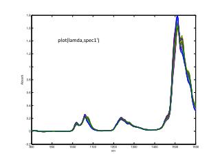
plot (lamda,spec1'). plot ( conc ). >> xc=spec1(1:20,:); >> xv=spec1(21:30,:); >> cc= conc (1:20,:); >> cv= conc (21:30 ,:); >> sp = pinv (cc)*xc; >> plot ( lamda,sp '). Calibration with all analytes (complete information ) ccp =xc* pinv ( sp ); cvp =xv* pinv ( sp );

E N D
>> xc=spec1(1:20,:); >> xv=spec1(21:30,:); >> cc=conc(1:20,:); >> cv=conc(21:30,:); >> sp=pinv(cc)*xc; >> plot(lamda,sp')
Calibrationwithallanalytes (complete information) ccp=xc*pinv(sp); cvp=xv*pinv(sp); lsreg2(cv(:,3),cvp(:,3)) slope offset corcoefsdres 9.8984e-01 7.1661e-02 9.9923e-01 7.3747e-01 aanalytermsepsepbiasrel.errorin % 3 4.1692e-01 2.5413e-01 3.4015e-01 1.0178e+00
b3=inv(xc'*xc)*xc'*cc(:,3); plot(b3)
>> ccp3=xc*b3; >> lsreg2(cc(:,3),ccp3) lsreg2(cc(:,3),ccp3) slopeoffset corcoefsdres 3.3996e+00 9.6790e+02 3.3060e-01 2.6693e+02 analytermsepsepbiasrel.error in % 1.0000e+00 1.0600e+03 6.3083e+01 -1.0583e+03 2.7781e+03
Calibrationwithonlyoneanalyte (incompleteinformation) >> ccp3=xc*pinv(sp(3,:)); >> cvp3=xv*pinv(sp(3,:)); lsreg2(cv(:,3),cvp3) slopeoffset corcoefsdres 2.9169e-01 6.9420e+01 9.2236e-01 2.3241e+00 analytermsepsepbiasrel.error in % 1.0000e+00 4.0950e+01 4.5576e+00 -4.0721e+01 9.9968e+01
lsreg2(cc(:,3),ccp3) slopeoffset corcoefsdres 1.0000e+00 -6.2741e-12 1.0000e+00 4.3581e-13 analytermsepsepbiasrel.error in 1.0000e+00 6.9601e-12 1.5403e-13 6.9585e-12 1.8241e-11
>> cvp3=xv*b3pinv; >> lsreg2(cv(:,3),cvp3) slopeoffset corcoefsdres 1.0007e+00 -4.3323e-02 9.9996e-01 1.6809e-01 analytermsepsepbiasrel.error in % 1.0000e+00 5.5101e-02 5.6219e-02 1.3842e-02 1.3452e-01
l=svd(spec1); l=l(1:10) l = 4.8019e+01 2.6726e+00 7.2263e-01 2.1746e-01 6.0301e-02 2.5724e-02 1.8327e-02 1.5100e-02 1.3410e-02 7.9763e-03 lambda selected lsel=[30,112,142,209,347];
>> xcr=xc(:,lsel); >> xvr=xv(:,lsel); b3r=inv(xcr'*xcr)*xcr'*cc(:,3); ccp3=xcr*b3r; cvp3=xvr*b3r; >> lsreg2(cv(:,3),cvp3) slopeoffset corcoefsdres 9.6617e-01 1.4917e+00 9.9920e-01 7.3588e-01 analytermsepsepbiasrel.errorin 1.0000e+00 3.3198e-01 3.2584e-01 -1.2105e-01 8.1044e-01
1) Centrado de los datos [xcm,xm]=mncn(xc); [ccm,cm]=mncn(cc); 2) Calibración Modelo PLS, calculo vector de regresión para el componente 3 [b3pls,ssq,p3,q3,w3,t3,u3,bin3] = pls(xcm,ccm(:,3),5,1); PercentVarianceCapturedby PLS Model -----X-Block----- -----Y-Block----- LV # This LV Total This LV Total ---- ------- ------- ------- ------- 1 91.88 91.88 86.62 86.62 2 6.97 98.85 8.07 94.69 3 0.93 99.78 4.63 99.31 4 0.19 99.96 0.63 99.94 5 0.02 99.98 0.02 99.96 4) Predcición en las muestras de validación del compuesto 3 con el modelo anterior cvp3pls5=xv m*b3pls(5,:)'; 5) Descentrado de la predición cvp3pls5m=rescale(cvp3pls5,cm(1,3));
6) Comprobación de la calidad de la predcción >> lsreg2(cv(:,3),cvp3pls5m) slope offset corcoefsdres 9.9526e-01 -2.0345e-01 9.9960e-01 5.3882e-01 analytermsepsepbiasrel.error in % 1.0000e+00 4.3161e-01 1.8210e-01 3.9553e-01 1.0537e+00