Download
1 / 111
1.4k likes | 2.03k Views
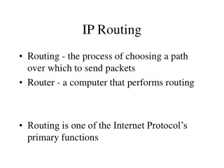
IP Routing. Section A : Introduction to IP Routing Section B : Routing Information Protocol (RIP) (Intra –AS), Open Shortest Path First (OSPF). Section C : CIDR, Inter-AS Routing: BGP (Inter-AS). Section A IP Routing. Routing: Process of choosing a path over which to send packets.

E N D
IP Routing Section A: Introduction to IP Routing Section B: Routing Information Protocol (RIP) (Intra –AS), Open Shortest Path First (OSPF). Section C: CIDR, Inter-AS Routing: BGP (Inter-AS)
Section AIP Routing • Routing: Process of choosing a path over which to send packets. • Routing occurs at TCP/IP host when it sends IP packets and at an intermediate IP router. • IP module central to Internet technology. • Essence of IP is its routing table. • IP uses this in-memory table to make all decisions about routing an IP packet.
Routing versus Forwarding • Forwarding: Taking a packet, looking at its DA, consulting the table, sending the packet accordingly on the right interface. • Routing: Process by which forwarding tables are built. • Complex distribution algorithms. • Forwarding Table versus Routing Table: Separate data structures for the two preferred. • Optimizing lookup, optimizing topology calculation.
Figure 1: Routing and Forwarding Tables Routing Table Forwarding Table
Routing Principles • Decision has to be made as to where the packet is to be forwarded. (router/host) • IP layer consults routing table in memory. • By default, a router can send packets only to networks to which it has configured interface. Communication Steps • IP first determines if destination host is local or on a remote network. (Applying subnet mask). • If remote, check routing table for a route to remote host or remote network.
Routing Principles • If no explicit route is found, IP uses default gateway address • At the default router, • Consult routing table, if a path is not found, use default gateway address • Process repeated, until packet finally delivered to destination host. • If route not found, error message sent to source. • an ICMP “host unreachable” or “network unreachable” is sent back to original sender.
Routing Methods • Methods necessary to make the size of routing table more manageable. Methods • Next-Hop • Network Specific • Host Specific • Default
Figure 2: Next Hop Routing Table holds only the address of the next hop Entries in the table consistent with each other. Table for R1 Table for R2 Table for Host A Dest Route Dest Route Dest Route B B B R2, B B R1, R2, B Host B Routing tables based on Route Host A R1 R2 Network Network Network Table for Host A Table for Host R1 Table for R2 Dest Next Hop DestNext Hop Dest Next Hop B R2 B R1 B Routing tables based on next hop
Figure 3: Network Specific/Host Specific Routing Routing table for host S based on host-specific routing Destination Next Hop A R1 B R1 C R1 D R1 Routing table for host S based on network specific routing Destination Next Hop N2 R1 S A B C D R1 N1 N2
Figure 4: Default Routing Destination Next Hop N2 R1 : : Default R2 Host A R1 N1 N2 Default Router R2 Rest of the Internet
Routing Table Routing table • IP performs the following steps when it searches its routing table: • Search for Direct delivery • Search for a matching host address. • Search for a matching network address. • Search for a default entry. Default entry normally specified in routing table as network entry, with a network ID of 0. • A matching host address is always used before a matching network address. (Refer to Table 3)
Figure 5: Example of a Routing Table Flags U: Up G: Gateway H: Host- Specific D: Added by redirection M: Modified by redirection 129.8.0.0 222.13.16.40 222.13.16.41 134.18.5.1 220.3.6.0 m1 m0 134.18.0.0 R3 R1 Rest of the Internet 134.18.5.2 R2 Routing Table for R1 Mask Destination Next Hop F RC U I 255.255.0.0134.18.0.0 U 0 0 m0 255.255.0.0 129.8.0.0 222.13.16.40 UG 0 0 m1 255.255.255.0 220.3.6.0 222.13.16.40 UG 0 0 m1 0.0.0.0 0.0.0.0 134.18.5.2 UG 0 0 m0
Routing Strategies Routing can either be static or dynamic. Static Routing • Require that routing tables are built and updated manually. Dynamic Routing • Routers update dynamically. • A function of routing protocols such as RIP and OSPF.
Figure 6: Configuring Static IP Routers Routing Table A 131.107.8.0 131.107.8.1 131.107.24.0 131.107.16.1 131.107.16.0 131.107.16.2 Routing table B 131.107.24.0 131.107.24.1 131.107.8.0 131.107.16.2 131.107.16.0 131.107.16.1 131.107.24.1 131.107.16.2 131.107.16.1 131.107.8.1 Multihomed computer N/W:131.107.24.z N/w: 131.107.8.z N/W: 131.107.16.z
Static Routing (Configuration) • A static routing table entry is created on computer A (Figure 14) • Network ID of network 3 • IP address (131.107.16.1) of the appropriate interface . • A static routing table entry is created on computer B • Network ID of network 1 • IP address (131.107.16.2) of appropriate interface. • Host’s default gateway address configured to match IP address of router’s local interface. • ‘Route’ command:Adds static entries to the routing table.
Dynamic Routing • Routers talk to adjacent routers • Informing each other of network status (Their view). • Routers communicate using a routing protocol • Many protocols to choose from. • Change in route: Automated change in routing table: Change in others routing tables. • Typically implemented on large internetworks • Minimal configuration is required by network administrator.
Autonomous Systems • Internet: Collection of autonomous systems (AS) each of which is administered by a single entity. • Example: A corporation or a university campus. • Each AS select its own routing protocol to communicate between routers in that AS. (Intra AS Routing) • Example: RIP and OSPF. • Separate routing protocols used between routers in different ASs. Example: BGP (Border Gateway Protocol). • (Inter-AS Routing)
Routing Strategies in Autonomous Systems Distance Vector Routing • Knowledge about the whole network. • Routing only to neighbours. • Information sharing at regular intervals. • Cost: In terms of hops. Example: RIP Link State Routing • Knowledge about neighbourhood. • To all routers. • Information shared at regular intervals. • Cost: On variety of factors. Example OSPF.
Routing Algorithms • Routing Algorithm: Part of network layer software responsible for deciding which output line an incoming packet should be transmitted on: Properties of routing algorithm • Correctness and simplicity • Robustness • Stability • Fairness and optimality Routing Algorithms • Adaptive • Non-adaptive
Figure 7: Fairness and Optimality Conflict B C A X’ X C’ A’ B’
Types of Routing Algorithms • Flooding • Distance Vector Routing (Discussed under RIP) • Link State Routing • Hierarchical Routing • Broadcast Routing
Flooding • Every incoming packet sent out on every outgoing line except the one arrived on. • Generation of vast amount of duplicate packets. • Solution • Hop Counter • Sequence Number: List maintenance
Hierarchical Routing • Routers are divided into regions. (Figure 2) • Each router knows all details on how to route packets within its own region. • Router knows nothing of internal structure of other regions. • For huge networks, two-level hierarchy insufficient. • Regions grouped into clusters, clusters into zones and so on. • Advantage: Reduction of entries in routing table. • Problem: Increased path length
Figure 8: Hierarchical Routing 1B 2A 2B 1A 1C Region 1 Region 2 2C 2D 5B 4A 5C 5A 3A 3B 5D 4B 5E 4C Region 3 Region 4 Region 5
1A - - 1B 1B 1 1C 1C 1 2A 1B 2 2B 1B 3 2C 1B 3 2D 1B 4 3A 1C 3 3B 1C 2 4A 1C 3 4B 1C 4 4C 1C 4 5A 1C 4 5B 1C 5 5C 1B 5 5D 1C 6 5E 1C 5 Table 1: Routing Table for 9A (No Hierarchical Routing) Dest. Line Hops Dest. Line Hops
Table 2: Hierarchical Table for 9B Dest. Line Hops
Broadcast Routing • Broadcasting: Sending a packet to all destinations simultaneously. • Schemes: • Flooding. • Multi-destination Routing. • Spanning Tree.
Routing Information Protocol (RIP) • RFC 1058 (RIPv1), RFC 2453 (RIP V2) • Original routing protocol of Xerox Network Services (XNS) protocol suite. • UC Berkeley adapted RIP for TCP/IP, Novell Inc. adapted it for Netware. This led to its widespread use. • Uses distance vector algorithm to compute routes • RIP enabled routers exchange network ids of networks the routers can reach • Hop Count: Number of routers crossed to reach desired network ID
RIP The broadcast of RIP packets allows: • workstations to locate the fastest route to a network number. • routers to request routing information from other routers to update their own internal tables. • Routers respond to route requests from workstations/other routers. • Broadcast make sure: • All routers are aware of internetwork configuration.
Distance Vector (Bellman-Ford) Routing • RIP uses distance vector routing to keep a list of all known routes in the routing table. • When it boots, router initialises its routing table to contain an entry for each directly connected network. • Each entry in the table identifies a destination network and gives distance to that network. • It also contains a hop count and a next hop field. • The routing table is updated upon receipt of a RIP response message.
Distance Vector Routing 3 steps in this algorithm: • Sharing knowledge about the entire autonomous system. • Sharing only with neighbours. • Sharing at regular intervals.
Figure 9: RIP Routing Table Destination Hop Count Next Hop Other Information
Distance Vector Routing • Add one hop to hop count for each advertised destination. • Repeat following steps for each advertised destination: • If destination not in routing table • Add advertised information in the routing table. • Else • If Next-hop field is same • Replace entry in table with advertised one. • Else • If advertised hop count smaller than one in routing table • Replace entry in routing table.
Distance Vector Routing Algorithm so far sends update message every 30 seconds. Metric in update message < metric in router’s table, Updating done. Update from next hop indicates different metric: Metric changes. Guarantees good performance but not good enough. This algorithm leads to “counting to infinity” problem. RIP: Maximum hop count: 15:anything greater considered unreachable.
RIP message from C after Increment RIP Message form C Net2 4 Net2 5 Net3 9 Net3 8 Figure 10 Net6 5 Net6 4 Net8 4 Net8 3 Net9 6 Net9 5 Old Routing Table New Routing Table Net1 7 A Net1 7 A Updating Algorithm Net2 2 C Net2 5 C Net6 8 F Net3 9 C Net6 5 C Net8 4 E Net8 4 E Net9 4 F Net9 4 F
RIP Details RIP implementation keeps following information about destination Address: IP address of the host or network. Gateway: First gateway along the route to destination. Interface: The physical network which must be used to reach first gateway. Metric: A number indicating the distance to destination. Timer: Amount of time since the entry was last updated. RIP Message Types: Requests, Responses
Figure 11: RIP Packet Format (8) (8) Command Version 1 Reserved Family (16) All Os Network Address (14 Bytes) Repeated All 0s All 0s Distance (metric)
Figure 12: RIP Routing Table A Routing Table B Network Router Hops Network Router Hops 131.107.8.0 131.107.16.2 2 (Learned from RIP) 131.107.8.0 131.107.8.1 1 131.107.16.0 131.107.16.2 1 131.107.24.0 131.107.16.1 2 (Learned from RIP) 131.107.16.0 131.107.16.1 1 131.107.24.0 131.107.24.1 1 Router A Router B 131.107.16.2 131.107.8.1 131.107.24.1 131.107.16.1 Routing Information A B (For A: Default Gateway) 131.107.8.1) (For B: Default Gateway) 131.107.24.1) 131.107.16.z 131.107.24.z 131.107.8.z
Figure 13: RIP Timers Timers Periodic (25-35) seconds Garbage Collection 120 Seconds Expiration 180 Seconds
Figure 14: Count to Infinity Problem A B C D E 1 2 3 4 3 2 3 4 3 4 3 4 5 4 5 4 5 6 5 6 7 6 7 6 7 8 7 8 Initially After 1 exchange After 2 exchanges After 3 exchanges After 4 exchanges After 5 exchanges After 6 exchanges
Count to Infinity Problem • Refer to Figure 8. • Consider 5 node (linear) subnet, where delay metric is number of hops. • All lines and routers are up initially. • Routers B, C, D, E have distances to A of 1, 2, 3 and 4 respectively. • Suddenly A goes down. • At first packet exchange, B hears nothing from A. • C advertises a length of 2 from A. • Received by B.
Count to Infinity Problem • B not aware that C’s path runs through B itself. • B thinks it reaches A via C with path length of 3. • D and E do not update their entries for A on first exchange. • On the second exchange, C notices each of its neighbors (B, D) claims to have a path to A of length 3. • It picks any one at random, makes its new distance to A 4. • Subsequent exchanges produce history • Gradually, all routers work their way to infinity. • This is known as Count to Infinity problem
Count to Infinity Problem: Solutions • Triggered Updates: Change propagated immediately. • Split Horizon: Utilizes selectivity in the sending of routing messages. • Poison Reverse: A variation of split horizon.
Triggered Updates/Split Horizon • Triggered Updates: Metric change triggers update. • Update messages sent NOT at regular update messages. • Problem • Reduce chances to get “counting to infinity”. • However this can still happen Split Horizon • Distance to an entity X not reported on line that packets for X are sent. • Reported as infinity. Poison Reverse: Infinite Metric for incoming interface.
RIP Shortcomings • Limited : longest path involves 15 hops. • RIP broadcast carry large routing tables. • Maximum Packet size: 512 bytes • Multiple RIP packets sent. • Significant bandwidth amount reserved. • Uses fixed metrics to compare alternative routes. • Recovery from failure: slow Process. • During this time, routing loops may occur. • RIP has no knowledge of subnet addressing.
RIP Version 2 • An extension over RIP v1. • No augmentation of length. • Use of existing unused fields. • Overcomes some shortcomings of RIP version 1. • RIP version 1 and RIP version 2 can interoperate if RIP ignores the fields must be zero. • RIP Version 2 message format. • Supports authentication and Multicast (Address: 224.0.0.9) • Refer to the Figure 9.
Figure 15: RIP Version 2 Message Format Command Version Reserved Route Tag Family Network Address Subnet mask Next-Hop Address Distance
Link State Routing Open Shortest Path First (OSPF)
Open Shortest Path First • Interior Routing Protocol (RFC 2328). • Developed by the OSPF working group of the Internet Engineering Task Force. • Starting assumptions similar to those of distance vector routing. • Every node knows how to reach its directly connected neighbors. • Each participating node has enough information to find the least cost path to any destination. • Two mechanisms: • Reliable dissemination of link state information • Calculation of routes: sum of all accumulated link-state knowledge.
Routing Areas • Area: A technique to partition a routing domain into sub-domains. • Area Border Routers: Summarize the information about the area and send it to other areas. • Backbone Area: All other areas must be connected to the backbone. • Primary • Routers within areas can still be connected to each other.