Download
1 / 59
590 likes | 738 Views
CLARREO Langley IR Study: Numerical simulation. Bruce Wielicki 1 , Seiji Kato 1 , Fred Rose 2 , Dave Kratz 1 , Xu Liu 1 , Sunny San-Mack 2 , and Walt Miller 2 1 NASA Langley Research Center 2 Science Systems & Applications Inc. the First CLARREO Mission Study Team Meeting

E N D
CLARREO Langley IR Study:Numerical simulation Bruce Wielicki1, Seiji Kato1, Fred Rose2, Dave Kratz1, Xu Liu1, Sunny San-Mack2, and Walt Miller2 1NASA Langley Research Center 2Science Systems & Applications Inc. the First CLARREO Mission Study Team Meeting Newport News, Virginia April 30 to May 2, 2008
Ties to Traceability Matrix • Climate model OSSEs Optimal for studies related to impact of benchmark spectra on climate change detection, attribution, prediction accuracy, decade to 100 year time scales, clear vs all-sky simulations • Observation + RTM spectra simulations Optimal for studies of field of view (spatial variability < 100km scale), realistic interannual variability, realistic clouds, aerosols (e.g. A-train), issues of sampling/swath for a range of time/space scales, diurnal sampling studies.
Ties to Traceability Matrix • LaRC IR Studies Summary: • A-train + RTM for most realistic aerosol/cloud variability • Field of View, Cirrus + Trade Cu effects, Cloud Overlap, Spectral Coverage (e.g. Far-IR) • Line-by-Line studies of linearity of distributions of atmospheric properties to averaged spectra • Benchmark spectra relation to underlying climate signals • Intercalibration of broadband and imagers in solar and infrared (last workshop). • Field of view, Swath, Orbit, Pointing ability, knowledge, control • Full Swath vs Nadir Only Sampling using CERES surface, cloud, aerosol, radiation data. • Swath, Number of Orbits • Diurnal Sampling studies for climate change: CERES + 3-hrly geo data, vs CERES Terra 1030LT only • Orbits, Number of Orbits
Method • Step 1: Use simple clouds and atmosphere and a) test sensitivity of the TOA effective temperature (spectrum) to atmospheric and cloud properties b) test if we can infer atmospheric property changes from time series of spectrum anomalies. • Step 2: Use A-train realistic cloud fields, test our results from Approach 1.
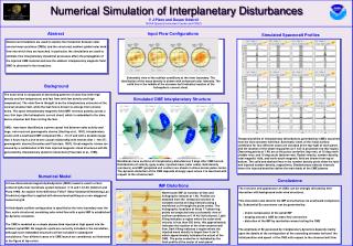
Realistic Cloud fields • Cloud fields are derived from CALIPSO, CloudSat, and MODIS (C3M), including thin cirrus, boundary layer cumulus, multi-layer clouds, and aerosols. • C3M product contains merged CALIPSO, CloudSat, CERES and MODIS data, SW and LW TOA flux from CERES, and flux profiles computed with CALIPSO, CloudSat, and MODIS clouds and aerosols (work is funded by NASA Energy Water Cycle Study (NEWS)
CloudSat Profile MODIS Pixel Calipso Shots 1.1 km 333 m 1 km 1.4 km MODIS Swath CALIPSO CloudSat MODIS collocation From S. Sun-Mack
Cloud and aerosol fields from 532 nm
Cloud cover over CALIPSO-CloudSat ground-track Clear-sky 6.1% 2.7% 15.0% 11.2%
Study with CALIPSO-CloudSat cloud fields • Compute TOA spectra with MODTRAN, Principal Component Radiative Transfer Model (PCRTM), and lbl code. • Examine whether or not atmospheric property changes can be detected from TOA spectra. • Examine whether or not signals can be separated when more than one variables change at the same time.
Averaging spectral data • Which atmospheric variables give a linear response to the brightness temperature at TOA? • Look for the mean spectra = spectrum of the mean • How does the linearity depend on the mean atmospheric state?
Hypothetical atmospheric property change • Assume a distribution of a cloud or an atmospheric property x at time t1. • Perturb the distribution for the distribution of x at time t2. • Compute mean spectrum from the distribution at t1 and t2 separately by weighting the spectrum by frequency of occurrence. • Compute the difference of the mean spectrum at t1 and t2: • Compute the mean of x at t1 and t2, two spectra using two mean values, and the difference
Black Blue Orange Simple study with MODTRAN Mean 0.98 1.01
Black Blue Orange Mean 10 km 12 km
Sensitivity Cloud height Emissivity = 1-exp(-tau*0.5) Water vapor Scale height Lapse rate (0 - 15 km) --> T(z) Skin temperature Surface air temperature (fixed QSH, RHSFC) -->H2O(z) Surface relative humidity (fixed QSH, TSFC) -->H2O(z)
Linearity Surface air temp. 300+-5K Cloud height 10+-1 km Cloud emissivity 0.4+-0.01 Surface skin temp. 300+-1K
Strategy • Use LBL code to validate MODTRAN and PCRTM (especially spectra with clouds). • MODTRAN and PCRTM run faster than LBL. PCRTM is more flexible with inputs.
Diurnal Cycles: Full 3-hourly vs Terra 1030LT onlyIs interannual variability in regional, zonal, and global fluxes captured accurately by just Terra 1030LT vs full 3-hourly data?How do the differences compare to expected climate forcing and response?GEO = CERES + GEO = 3-hourly DataNon-GEO = CERES Terra only = 1030 AM/PM only
Tropical and Global Mean Effect of Diurnal Cycle: Very Small GEO is CERES + 3-hourly Geo Diurnal Cycle, nonGEO = CERES Terra Only
Tropical and Global Mean Effect of Diurnal Cycle: Very Small GEO is CERES + 3-hourly Geo Diurnal Cycle, nonGEO = CERES Terra Only
Jan 2001 De-seasonalized SW Flux Anomaly Relative to 2001-2005 Avg (CERES Terra plus 3-hourly geostationary data for diurnal cycle)
Jan 2001 De-seasonalized SW Flux Anomaly Relative to 2001-2005 Avg (CERES Terra (1030LT) only for diurnal cycle)
Jan 2001 De-seasonalized SW Flux Anomaly Relative to 2001-2005 Avg (With and Without Geo: Effect of Diurnal Cycle is Small)
Jan 2001 De-seasonalized LW Flux Anomaly Relative to 2001-2005 Avg (CERES Terra plus 3-hourly geostationary data for diurnal cycle)
Jan 2001 De-seasonalized LW Flux Anomaly Relative to 2001-2005 Avg (CERES Terra (1030LT) only for diurnal cycle)
Jan 2001 De-seasonalized LW Flux Anomaly Relative to 2001-2005 Avg (With and Without Geo: Effect of Diurnal Cycle is Small)
Conclusions • Regional, Zonal, Global monthly and interannual variations of SW and LW fluxes examined • Compared 3-hourly vs Terra sunsynch 1030LT only • Used all-sky fluxes to include both clear and cloudy diurnal cycles (land, stratus, convection, desert, etc) • While regional differences can be large in the mean fields (“true” vs 1030LT), global differences are very small. • For anomalies (monthly, interannual, regional, zonal, global) “true” vs 1030LT showed very small differences, with the solar flux effects about 3 times as large as infrared • LW and SW anomalies from “true” vs 1030LT anomalies are much less than natural variability