Download
1 / 22
230 likes | 351 Views
Partially Resolved Numerical Simulation. CRTI-02-0093RD Project Review Meeting Canadian Meteorological Centre August 22-23, 2006. Introduction. Urban Environment in City Scale (~1 km range) Contains regions of massive separation, recirculation, and turbulent wakes, etc.

E N D
Partially Resolved Numerical Simulation CRTI-02-0093RD Project Review Meeting Canadian Meteorological Centre August 22-23, 2006
Introduction • Urban Environment in City Scale (~1 km range) • Contains regions of massive separation, recirculation, and turbulent wakes, etc. • Conventional RANS approach is unable to correctly simulate above application • Hybrid RANS/LES approach is needed
Hybrid RANS/LES approaches • Conventional approach • spatially filtered equations are solved in the LES region • time averaged equations are solved in the RANS region • Incompatibility of flow properties between two regions occurs • Partially Resolved Numerical Simulation (PRNS) • temporal filtered equations are solved in both the LES and RANS regions • A unified simulation approach that spans the spectrum from RANS towards LES and DNS
Partially Resolved Numerical Simulation • Basic Idea • RANS and LES have the same form of filtered transport equation • A unified model can be developed to determine the degree of modeling required to represent the unresolved turbulent stresses • This can be achieved in principle through the rescaling of RANS models
PRNS model • Modeling Approach • A PRNS model is obtained by multiplying a dimensionless resolution control function (FR)to a RANS model: • Depends on the physical resolution requirement, the model can serve as: • a RANS model (FR1) where all turbulence scales are modeled, or • provides no modeling (FR0) where all scales are resolved • In between these two limits, the model behaves like a LES-type subscale model where only the unresolved scales are modeled • The fidelity of PRNS depends on the value of FR as well as on the specific formulation of the model where
Formulation of resolution control function (FR) • Speziale (1998): • Batten et al. (2000): • Liu and Shih (2006):
Our Formulation of FR • Hsieh, Lien and Yee (2006): • Assume energy spectrum E() 2/3-5/3for ic k FR=0 FR=1 logE() log i c K
Implementation of FR • Method 1: • FR is only applied in momentum equations to reduce the magnitude of turbulent stresses from RANS-like calculation • k and are the large scale turbulent energy and dissipation rate • Adopted by Speziale (1998) and Hsieh, Lien and Yee (2006)
Implementation of FR • Method 2: • FR is applied in momentum and turbulence transport equations to reduce the amplitude of eddy viscosity • k and are the subscale scale turbulent energy and dissipation rate • Adopted by Batten et al. (2000) and Liu and Shih (2006)
Implementation of FR • Summary k, t=Ck2/ Method 1: Method 2:
Reynolds stresses calculation in PRNS • Reynolds stresses • has contributions from both the resolved and unresolved scales • Reconstruction of modeled Reynolds stresses • To use PRNS calculation on a RANS-type coarse grid, a new formulation which require the reconstruction of is proposed • An ad hoc modeled Reynolds stresses is introduced, where the non-linear effect of subscale stresses are absorbed into FR • The optimal value of the exponent n needs to be determined over a range of flow conditions, and currently n=0.3 is used
Test case • Case 6.2 • Fully developed channel flow over a matrix of 250 wall-mounted cubes (Meinders and Hanjalic, 1999) • Benchmark problem for the 8th ERCOFTAC workshop (1999)
Results • Numerical results are obtained based on: • 45x45x45 nodes (streamwise by spanwise by vertical) • Standard k- turbulence model with wall functions are used for URANS and PRNS calculations
Time History at (x,y,z) = (0.5, 1.3, 0)
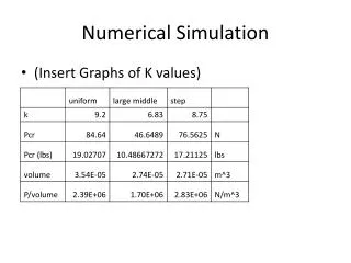
Energy Spectrum at (x,y,z) = (0.5, 1.3, 0)
Conclusions • PRNS provides a unified simulation strategy for high Reynolds number complex turbulent flows • Implementation of PRNS to any CFD code that runs URANS simulation is straightforward and requires very minimum modifications • PRNS has been demonstrated in improving the prediction of turbulent mean quantities
References • Batten, P., Goldberg, U., and Chakravarthy, S. (2000), “Sub-grid turbulence modeling for unsteady flow with acoustic resonance”, AIAA paper 2000-0473. • Hellsten, A., Rautaheimo, P. (1999). “Workshop on refined turbulence modelling”, Proceedings of the 8th ERCOFTAC/IAHR/COST Workshop, 17–18 June, 1999, Helsinki, Finland. Helsinki University of Technology. • Meinders E.R. and Hanjalic K. (1999), “Vortex structure and heat transfer in turbulent flow over a wall-mounted matrix of cubes”, Int. J. Heat Fluid Flow, Vol. 20, pp. 255-267. • Liu N.S. and Shih T.H. (2006), “Turbulence modeling for very large-eddy simulation”, AIAA Journal, Vol.44, pp. 687-697. • Speziale, C.G. (1998), “Turbulent modeling for time-dependent RANS and VLES: a review”, AIAA Journal, Vol. 36, pp. 173-184.