Download
1 / 14
160 likes | 423 Views
Magnetic Fields & Numerical Simulation. Madhawa Hettiarachchi, PhD LPPD Director Prof. Andreas A. Linninger 09/02/2010. Maxwell’s equations. Ampere’s Law- Magnetic field can be generated by both electrical current and changing electric fields.

E N D
Magnetic Fields & Numerical Simulation Madhawa Hettiarachchi, PhD LPPD Director Prof. Andreas A. Linninger 09/02/2010
Maxwell’s equations Ampere’s Law- Magnetic field can be generated by both electrical current and changing electric fields The total magnetic flux through any Gaussian surface is zero Faraday’s Law -magnetic flux density [V/m] -magnetic field intensity [W/m2, T] -electric field intensity [V/m] -electric flux density [W/m2] -current density [A/m2] -electric charge density[C/m2] -permeability [H/m] -permittivity [F/m] Gauss's Law Constitutive equations
Numerical Solution Method • Current system of equations lead to parabolic PDE form • We would like to formulate the Maxwell’s equations similar to diffusion and convention transport. • This will let us to use Finite-volume numerical approach to solve the Maxwell’s system of equations and more importantly it will give us greater insight in to the understanding of electromagnetic fields. • By considering magnetic and electric fields as potential fields, we can transform the Maxwell’s equations into the desired form.
Magnetic Vector Potential - Magnetic vector potential V – Electrical scalar potential is a vector quantity that mathematically acts like a potential, in that we can obtain the magnetic field from it by taking the derivative. Vector identity Curl of the gradient of any scalar field is always the zero vector. Divergence of the curl of any velocity field is zero.
Magnetic Vector Potential A - magnetic vector potential V – Electrical scalar potential Satisfy from the vector identity 0
Static Magnetic Fields -Magnetic field generated by a permanent magnet -Simplified Maxwell’s equations: Magnetic scalar potential, A, is defined as, Similar to Diffusion equation 0 Vector identity theory -Static magnetic field potential behaves similar to diffusion of a species.
Analogy between electric & magnetic fields and diffusion/conduction
Test case: Static Magnetic Fields -Unstructured mesh –bent knee -Dirichlet boundary condition, -Nuemann boundary condition,
Arrows shows the gradient of the potential at the cell face centers ,Magnetic potential Static Magnetic Fields
Magnetic potential field Conduction problem ,Temperature ,Magnetic potential
More realistic case: -Nuemann Boundary condition
,Magnetic potential ,Magnetic potential
Point Magnet ,Magnetic potential
Next step • Magnetic nanoparticles for targeted drug delivery • Force on the nanoparticles by the magnetic field • Diffusion of the nonoparticles • Convection and diffusion of the bulk fluid