Download
1 / 37
370 likes | 418 Views
This lecture covers microarray data analysis methods, such as hierarchical and K-means clustering, to extract gene functionality from expression data. It discusses the significance of interpreting gene expressions and provides insights into various techniques. Discover how microarrays revolutionize gene function inference through advanced data analysis.

E N D
Microarray Data Analysis (Lecture for CS498-CXZ Algorithms in Bioinformatics) Oct 13, 2005 ChengXiang Zhai Department of Computer Science University of Illinois, Urbana-Champaign
Outline • Microarrays • Hierarchical Clustering • K-Means Clustering • Corrupted Cliques Problem • CAST Clustering Algorithm
Motivation: Inferring Gene Functionality • Researchers want to know the functions of newly sequenced genes • Simply comparing the new gene sequences to known DNA sequences often does not give away the function of gene • For 40% of sequenced genes, functionality cannot be ascertained by only comparing to sequences of other known genes • Microarrays allow biologists to infer gene function even when sequence similarity alone there is insufficient to infer function.
Microarrays and Expression Analysis • Microarrays measure the activity (expression level) of the genes under varying conditions/time points • Expression level is estimated by measuring the amount of mRNA for that particular gene • A gene is active if it is being transcribed • More mRNA usually indicates more gene activity
Microarray Experiments • Produce cDNA from mRNA (DNA is more stable) • Attach phosphor to cDNA to see when a particular gene is expressed • Different color phosphors are available to compare many samples at once • Hybridize cDNA over the micro array • Scan the microarray with a phosphor-illuminating laser • Illumination reveals transcribed genes • Scan microarray multiple times for the different color phosphor’s
Microarray Experiments (con’t) Phosphors can be added here instead Then instead of staining, laser illumination can be used www.affymetrix.com
Interpretation of Microarray Data • Green: expressed only from control • Red: expressed only from experimental cell • Yellow: equally expressed in both samples • Black: NOT expressed in either control or experimental cells
Microarray Data • Microarray data are usually transformed into an intensity matrix (below) • The intensity matrix allows biologists to make correlations between different genes (even if they are dissimilar) and to understand how gene functions might be related • Clustering comes into play Intensity (expression level) of gene at measured time
Major Analysis Techniques • Single gene analysis • Compare the expression levels of the same gene under different conditions • Main techniques: Significance test (e.g., t-test) • Gene group analysis • Find genes that are expressed similarly across many different conditions (co-expressed genes -> co-regulated genes) • Main techniques: Clustering (many possibilities) • Gene network analysis • Analyze gene regulation relationship at a large scale • Main techniques: Bayesian networks, won’t be covered
Clustering of Microarray Data Clusters
Homogeneity and Separation Principles • Homogeneity: Elements within a cluster are close to each other • Separation: Elements in different clusters are further apart from each other • …clustering is not an easy task! Given these points a clustering algorithm might make two distinct clusters as follows
Bad Clustering This clustering violates both Homogeneity and Separation principles Close distances from points in separate clusters Far distances from points in the same cluster
Good Clustering This clustering satisfies bothHomogeneity and Separation principles
Clustering Methods • Similarity-based (need a similarity function) • Construct a partition • Agglomerative, bottom up • Typically “hard” clustering • Model-based (latent models, probabilistic or algebraic) • First compute the model • Clusters are obtained easily after having a model • Typically “soft” clustering
Similarity-based Clustering • Define a similarity function to measure similarity between two objects • Common clustering criteria: Find a partition to • Maximize intra-cluster similarity • Minimize inter-cluster similarity • Challenge: How to combine them? (many possibilities) • How to construct clusters? • Agglomerative Hierarchical Clustering (Greedy) • Need a cutoff (either by the number of clusters or by a score threshold)
Method 1 (Similarity-based):Agglomerative Hierarchical Clustering
Similarity Measures • Given two gene expression vectors, X={X1, X2, …, Xn} and Y={Y1, Y2, …, Yn}, define a similarity function s(X,Y) to measure how likely the two genes are co-regulated/co-expressed • However “co-expressed” is hard to quantify • Biology knowledge would help • In practice, many choices • Euclidean distance • Pearson correlation coefficient Better measures are possible (e.g., focusing on a subset of values…
Agglomerative Hierachical Clustering • Given a similarity function to measure similarity between two objects • Gradually group similar objects together in a bottom-up fashion • Stop when some stopping criterion is met • Variations: different ways to compute group similarity based on individual object similarity
Hierarchical Clustering Algorithm • Hierarchical Clustering (d, n) • Form n clusters each with one element • Construct a graph T by assigning one vertex to each cluster • while there is more than one cluster • Find the two closest clusters C1 and C2 • Merge C1 and C2 into new cluster C with |C1| +|C2| elements • Compute distance from C to all other clusters • Add a new vertex C to T and connect to vertices C1 and C2 • Remove rows and columns of d corresponding to C1 and C2 • Add a row and column to d corrsponding to the new cluster C • return T The algorithm takes a nxn distance matrix d of pairwise distances between points as an input.
Hierarchical Clustering Algorithm • Hierarchical Clustering (d, n) • Form n clusters each with one element • Construct a graph T by assigning one vertex to each cluster • while there is more than one cluster • Find the two closest clusters C1 and C2 • Merge C1 and C2 into new cluster C with |C1| +|C2| elements • Compute distance from C to all other clusters • Add a new vertex C to T and connect to vertices C1 and C2 • Remove rows and columns of d corresponding to C1 and C2 • Add a row and column to d corrsponding to the new cluster C • return T Different ways to define distances between clusters lead to different clustering methods…
How to Compute Group Similarity? Three Popular Methods: Given two groups g1 and g2, Single-link algorithm: s(g1,g2)= similarity of the closest pair complete-link algorithm: s(g1,g2)= similarity of the farthest pair average-link algorithm: s(g1,g2)= average of similarity of all pairs
complete-link algorithm g2 g1 ? …… Single-link algorithm average-link algorithm Three Methods Illustrated
Group Similarity Formulas • Given C (new cluster) and C* (any other cluster in the current results) • Given a similarity function s(x,y) (or equivalently, a distance function, d(x,y) as in the book) • Single link: • Complete link: • Average link:
Comparison of the Three Methods • Single-link • “Loose” clusters • Individual decision, sensitive to outliers • Complete-link • “Tight” clusters • Individual decision, sensitive to outliers • Average-link • “In between” • Group decision, insensitive to outliers • Which one is the best? Depends on what you need!
A Model-based View of K-Means • Each cluster is modeled by a centroid point • A partition of the data V={v1…vn}with k clusters is modeled by k centroid points X={x1…xk}; Note that a model X uniquely specifies the clustering results • Define an objective function on X and V to measure how good/bad V is as clustering results of X, f(X,V) • Clustering is reduced to the problem of finding a model X* that optimizes the value f(X*,V) • Once X* is found, the clustering results are simply computed according to our model X* • Major tasks: (1) define d(x,v); (2) define f(X,V); (3) Efficiently search for X*
Squared Error Distortion • Given a set of n data pointsV={v1…vn} and a set of k points X={x1…xk} • Define d(xi,vj)=Euclidean distance • Define f(X,V)=d(X,V) (Squared error distortion) The distance from vi to the closest point in X
K-Means Clustering Problem: Formulation • Input: A set, V, consisting of n points and a parameter k • Output: A set X consisting of k points (cluster centers) that minimizes the squared error distortion d(V,X) over all possible choices of X This problem is NP-complete.
K-Means Clustering • Given a distance function • Start with k randomly selected data points • Assume they are the centroids of k clusters • Assign every data point to a cluster whose centroid is the closest to the data point • Recompute the centroid for each cluster • Repeat this process until the distance-based objective function converges
K-Means Clustering: Lloyd Algorithm • Lloyd Algorithm • Arbitrarily assign the k cluster centers • while the cluster centers keep changing • Assign each data point to the cluster Ci (xi) corresponding to the closest cluster representative (i.e,. the center xi) (1 ≤ i ≤ k) • After the assignment of all data points, compute new cluster representatives according to the center of gravity of each cluster, that is, the new cluster representative is *This may lead to merely a locally optimal clustering.
x1 x2 x3
x1 x2 x3
x1 x2 x3
x1 x2 x3
Evaluation of Clustering Results • How many clusters? • Score threshold in hierarchical clustering (need to have some confidence in the scores) • Try out multiple numbers, and see which one works the best (best could mean fitting the data better or discovering some known clusters) • Quality of a single cluster • A tight cluster is better (but needs to quantify the “tightness”) • Prior knowledge about clusters • Quality of a set of clusters • Quality of individual clusters • How well different clusters are separated • In general, evaluation of clustering and choosing the right clustering algorithms are difficult • But the good news is that significant clusters tend to show up regardless what clustering algorithms to use
What You Should Know • Why clustering microarray data is interesting • How hierarchical agglomerative clustering works • The 3 different ways of computing the group similarity/distance • How k-means works