Download
1 / 23
260 likes | 421 Views
Poisson processes. Stochastic Process By TMJA Cooray. Introduction. The probability models we have discussed so far involves random variables occurring in discrete sequence. That is both the random variable and the time parameter have been discrete.

E N D
Poisson processes Stochastic Process By TMJA Cooray
Introduction • The probability models we have discussed so far involves random variables occurring in discrete sequence. • That is both the random variable and the time parameter have been discrete. • Here we shall consider random variables in continuous time. MA (4030) Level 4-Poisson Processes
We introduce the basic stochastic model for events that occur at random moments in continuous time. • This model is called the Poisson Process • Examples: telephone calls arriving, emission of radio active atoms, occurrence of accidents, cosmic rays arriving etc. MA (4030) Level 4-Poisson Processes
Let the discrete random variable X(t): represents the size of the population being considered at any instant of time t. • Denote the probability that the population size at time t is n, as: MA (4030) Level 4-Poisson Processes
Memory less random variables • There’s a bin full of integrated circuit chips of a particular type. • Consider the random variable :The total operating time X of a single chip. • Assume that all the chips were manufactured under identical conditions ,so that the distribution of X is the same for all the chips. there are no faulty chips in the bin • X is a continuous r.v. and P[X>0]=1. MA (4030) Level 4-Poisson Processes
Consider the following scenario: • Select a chip at random from the bin install it and turn it on at time t=o. the probability that it is still operating at time t is P[X>t]. • Unplug the switch while its still working , after t hours of use. • Take the same chip and install it. • What is the pr. that chip will still be working after s hours of use in the second installation? • The conditional pr. P[X>s+t|X>t]=? MA (4030) Level 4-Poisson Processes
For many types of electronic equipments • P[X> s+t |X>t]= P[X>s] • A r.v. X≥0 satisfying the above equation for all s≥0 and t≥0 is said to have no memory. • Theorem :If X≥0 is a r.v. satisfying the above equation then X is an exponential r.v. with parameter . Conversely, every exponential r.v. satisfies the above equation . MA (4030) Level 4-Poisson Processes
Consider a very small time interval Δt, Probability of no failure during time t+Δt, when it has worked for time t • Probability of one failure during time t+Δt, when it has worked for time t Probability of more than one failure no failure during time t+Δt, when it has worked for time t • P[X>t+ Δt |X>t]= P[X> Δt] =e - Δt, • P[X<t+ Δt |X>t]= P[X< Δt] =1-e - Δt, MA (4030) Level 4-Poisson Processes
Poisson Process • Let X(t) be the total number of events (telephone calls) recorded up to time t. • This total number of calls is the population size in question. • It is usual to assume that the events involved occur at“random” • That is the chance of a new call arriving in any short interval is independent, not only of the previous state of the system ,but also of present state of the system.. MA (4030) Level 4-Poisson Processes
We can therefore assume that • The chance of a new addition to the total count ( a new call) during a very short interval of time Δt can be written as Δt +o(Δt ), where is average number of calls per unit time (which is some suitable constant characterizing the intensity of calls). • The chance of two or more calls during the very short interval of time Δt can be written as o(Δt ), • The chance of no call during a very short interval of time Δt can be written as 1- Δt +o(Δt ), MA (4030) Level 4-Poisson Processes
Then the probability of getting n calls up to time t +Δt are :, • Ignoring the small terms ( higher powers of small Δt ). • If n>0 ,this can arise in 2 ways. : n calls up to time (0,t) and no calls in time (t,t+Δt) : n-1 calls up to time (0,t) and one call in time (t,t+Δt) MA (4030) Level 4-Poisson Processes
Now it follows from 2, For n=0, n=0 at time t+Δt , only if n=0 at time t and no new calls are coming in Δt .In this case we can write: MA (4030) Level 4-Poisson Processes
If we start at time 0 with a new telephone or with a new record, • The set of differential- difference equations (3) and (4), together with the boundary condition (5) determines the probability distribution Pn(t). • Solving (4) log(p0(t))=- t+c using (5) c=0 giving , p0(t)= e -t ---------(6) Substituting this in (3),with n,=1 , gives p1(t)= t e -t MA (4030) Level 4-Poisson Processes
Repeating this procedure the following general formula can be obtained. This is simply a Poisson distribution with parameter t MA (4030) Level 4-Poisson Processes
This set of differential-difference equations given in (3) can be solvedusing generating functions also. • Recall the probability generating functions p(x,t) for the probability distribution pn(t) • where p(x,t) is a function of t as well as x. MA (4030) Level 4-Poisson Processes
(9) involves differentiation in t only and,can be integrated directly in conjunction with (10), to obtain • this is immediately identifiable as The probability generating function of a Poisson distribution with parameter t, the individual probabilities given by (7) MA (4030) Level 4-Poisson Processes
Partial differential-difference equation (10) can be written for the moment generating function M(,t),merely by putting x=e, giving • In different situations one generating function may be easily soluble than the other. MA (4030) Level 4-Poisson Processes
Solution of linear Partial differential equations. • For many processes ,,these generating functions are linear functions of the differential operators • in order to solve them ,the main results that we shall require are given as follows. MA (4030) Level 4-Poisson Processes
Consider the linear partial differential equation: • subject to some appropriate boundary conditions ,where P,Q and R may be functions of x,y and z.first step is to form the subsidiary equations given by : MA (4030) Level 4-Poisson Processes
We can find two independent integrals of these subsidiary equations ,writing them in the form , u(x,y,z)= constant, v(x,y,z)=constant ...(16) • The most general solution of (13) is now given by (u,v)=0 • u=(v) ........ (17) • where and are arbitrary functions.The precise form of these functions can be determined by using boundary conditions. MA (4030) Level 4-Poisson Processes
Note:relationship between Poisson and (negative) exponential • If all the assumptions hold as for a Poisson process : • probability of no occurrence during a time interval (0,t) = p0(t)= e -t • That is the time interval between two consecutive occurrences ( a r.v.T) is >t. • P[T>t]= e -t ,Then P[T t]=1- e -t MA (4030) Level 4-Poisson Processes
which is the cumulative distribution F(t) of the r.v. T [the time interval between two consecutive occurrences ( or the inter arrival time)]. • Then P[T t] =F(t)=1- e -t • to find the corresponding density function differentiating F(t), we get F’(t)=f(t)= e -t , 0<t • which is the negative exponential distribution. MA (4030) Level 4-Poisson Processes