Download
1 / 45
730 likes | 1.39k Views
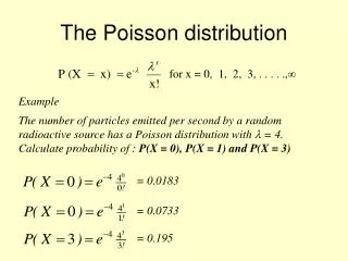
Poisson Distribution. Poisson. Poisson 1781-1840. Definition. The Poisson distribution is a discrete probability distribution.

E N D
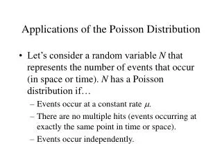
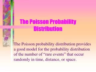
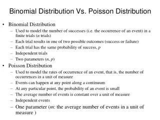
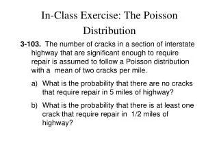
Definition • The Poisson distribution is a discrete probability distribution. • It expresses the probability of a number of events occurring in a fixed time if these events occur with a known average rate and are independent of the time since the last event.
Examples • The number of emergency calls received by an ambulance control in an hour. • The number of vehicles approaching a motorway toll bridge in a five-minute interval. • The number of flaws in a metre length of material.
Assumptions • Each occurs randomly. • Events occur singly in a given interval of time or space. • The mean number of occurrences in the given interval, is known and finite.
Example 1 • A student finds that the average number of amoebas in 10 ml of pond water from a particular pond is four. Assuming that the number of amoebas follows a Poisson distribution. • Find the probability that in a 10 ml sample • a) there are exactly five amoebas. • b) There are no amoebas • c) There are fewer than three amoebas.
a) Find the probability that in a 10 ml sample there are exactly five amoebas.
b) Find the probability that in a 10 ml sample there are no amoebas
c) Find the probability that in a 10 ml sample there are fewer than three amoebas.
Graphics Calc Poisson Dist For cumulative select Pcd after Poisn Stats Mode from Calc F5 Distribution Then F6 next F1 Poisn For P(X<3), For point dist select Ppd Select Data: Variable For P(X=1), For P(X=1) = 0.1494 Since tables only go to 4 dp, round to 4dp
Note the following: • 1. The binomial distribution is affected by the sample size and the probability while the Poisson distribution is ONLY affected by the mean. • 2. The binomial distribution has values from x = 0 to n but the Poisson distribution has values from x = 0 to infinity.
Example: On average there are three babies born a day with hairy backs. • Find the probability that in one day two babies are born hairy. • Find the probability that in one day no babies are born hairy.
Find the probability that in one day two babies are born hairy. Probability = 0.2240 Using formula sheet
Find the probability that in one day no babies are born hairy. Probability = 0.0498 Using formula sheet
Example: Suppose a bank knows that on average 60 customers arrive between 10 A.M. and 11 A.M. daily. • Find the probability that exactly two customers arrive in a given one-minute time interval between 10 and 11 A.M.
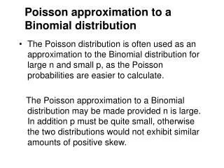
Compare Binomial to Poisson When probability is close to 1, Poisson can approximate the Binomial.
Approximation: If p is small, then the Binomial distribution with parameters n and p is well approximated by the Poisson distribution with parameter np, i.e. by the Poisson distribution with the same mean
Example Binomial situation, n= 100, p=0.075 Calculate the probability of fewer than 10 successes.
Probability = 0.7833 This would have been very tricky with manual calculation as the factorials are very large and the probabilities very small
The Poisson approximation to the Binomial states that will be equal to np, i.e. 100 x 0.075 so =7.5 Probability = 0.7764 So it is correct to 2 decimal places. Manually, this would have been much simpler to do than the Binomial.
Eggs are packed into boxes of 500. On average 0.7% of the eggs are found to be broken when the eggs are unpacked. Find the probability that in a box of 500 eggs • Exactly three are broken. • At least two are broken.
Eggs are packed into boxes of 500. On average 0.7% of the eggs are found to be broken when the eggs are unpacked. Find the probability that in a box of 500 eggs • Mean = 500 x 0.007 = 3.5
Eggs are packed into boxes of 500. On average 0.7% of the eggs are found to be broken when the eggs are unpacked. Find the probability that in a box of 500 eggs At least two are broken.
A Christmas draw aims to sell 5000 tickets, 50 of which will win a prize. A syndicate buys 200 tickets. Justify the use of a Poisson distribution. Probability is close to zero Strictly speaking, you don’t have independent trials, but n is very large.
A Christmas draw aims to sell 5000 tickets, 50 of which will win a prize. A syndicate buys 200 tickets. Calculate
A Christmas draw aims to sell 5000 tickets, 50 of which will win a prize. A syndicate buys 200 tickets. Calculate how many tickets should be bought in order for there to be a 90% probability of winning at least one prize.
A Christmas draw aims to sell 5000 tickets, 50 of which will win a prize. A syndicate buys 200 tickets. Calculate how many tickets should be bought in order for there to be a 90% probability of winning at least one prize. N must be 231
Two identical racing cars are being tested on a circuit. For each car, the number of mechanical breakdowns can be modelled by the Poisson distribution with a mean of one breakdown in 100 laps. If a car breaks down it is attended and continues on the circuit. The first car is tested for 20 laps and the second for 40 laps. Find the probability that the service team is called out to attend to breakdowns. Once More than twice
Two identical racing cars are being tested on a circuit. For each car, the number of mechanical breakdowns can be modelled by the Poisson distribution with a mean of one breakdown in 100 laps. If a car breaks down it is attended and continues on the circuit. The first car is tested for 20 laps and the second for 40 laps. Since the average number of breakdowns in 100 laps is one, the average in 20 laps is 0.2 and in 40 laps it is 0.4.
Two identical racing cars are being tested on a circuit. For each car, the number of mechanical breakdowns can be modelled by the Poisson distribution with a mean of one breakdown in 100 laps. If a car breaks down it is attended and continues on the circuit. The first car is tested for 20 laps and the second for 40 laps.
Poisson Approximation: the Birthday Problem. What is the probability that in a gathering of k people, at least two share the same birthday?
Suppose there are n days in the year (on Earth we have n = 365) Assume that each person has a birthday which is equally likely to fall on any day of the year, independently of the birthdays of the remaining k - 1 persons (no sets of twins in the group).
Then a simple conditional probability calculation shows that pn;k = 1- p(all birthdays are different) =
So that (on Earth) 23 is the minimum size of gathering required for a better than evens chance of two members sharing the same birthday. Proof of this The mean number of birthday coincidences in a sample of size k is:
The number of birthday coincidences should have an approximately Poisson distribution with the above mean. Thus, to determine the size of gathering required for an approximate probability p of at least one coincidence, we should solve
In other words we are solving the simple quadratic equation In the case n=365, p=0.5, this gives k=23.0
Notice as values ofincrease, the distribution becomes normally distributed.