EEE324 Digital Electronics

1. EEE324 Digital Electronics Lecture 4:Boolean Algebra Ian McCrum Room 5B18, 02890366364 IJ.McCrum@ulster.ac.uk http://www.eej.ulst.ac.uk/~ian/modules/EEE342

2. a variable is a symbol, for example , used to represent a logical quantity, whose value can be 0 or 1. • the complement of a variable is the inverse of a variable and is represented by an over bar, for example . • a literal is a variable or the complement of a variable. • Boolean Addition ( + ) • is equivalent to the OR operation; if any of the inputs are 1 then the output is also 1. • In Boolean algebra a sum term is a sum of literals. In a logic circuit a sum term is produced by an OR operation with no AND operations involved, for example . • Boolean Multiplication ( * ) or ( . ) Sometimes even the dot is left out. It is equivalent to the AND operation; if all of the inputs are 1 then the output is 1. • In Boolean algebra a product term is the product of literals. In a logic circuit a product term is produced by an AND operation with no OR operations involved, for example .

3. The 3 Laws of Boolean Algebra • the Commutative Laws • the Associative Laws • the Distributive Law

4. The 12 Rules of Boolean Algebra

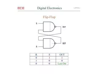
5. DeMorgans’ Theorems In graphical terms, Theorem 1 says you can replace a NAND gate with an OR gate that has invertors at its input. Sometimes we draw schematics with the alternate form, you will meet both. (look in the quartus libraries at the BNOR and BNAND gates.

6. Simplification using Boolean Algebra • Good designers make good designs; the “goodness” of a design can depend on many factors, • Cost; but this can be related to silicon area, power consumption, number of gates, number of different gates, number of packages, number of connections, cost of test… • A simple cost model might be 1p per input of gates with 2 or more inputs. (and 6 or 9p for storage devices, yet to be met)

7. Minimising Logic • With the rules of boolean algebra we can convert one logical expression into another • In practice we prefer two level AND-OR logic; this maps onto truth tables and algebraic expressions more naturally • There are also advantages in terms of time delays and gates counts. • However, if we have to fit a problem into a strange device we might need to refactor our expressions into an alternate form, for example Ferranti ULA devices only have NOR gates within them!

8. Example

9. Minimising using algebra

10. The Logic adjacency theorem • Rather than using one of 3 rules and one of 12 identities we can avail of a theorem that says • The logic adjacency theorem, correctly applied is all you need to guarantee a minimum solution is the logic adjacency theorem • And of course you need to know the logic adjacency theorem. • The phrase “correctly applied” is relevant when we have to apply the theorem multiple times and there is a choice as to which pair of terms to work on first; the order matters. • For simple problems a graphical technique can show us all possible applications of the adjacency theorem; it helps us choose an optimum covering. • If the problem is large then an exhaustive solution it impractical, near optimum results can be obtained by computer – the espresso software from Berkeley is a good example of this. (Quartus uses it)

11. The adjacency theorem If two literals differ in having one variable in the normal form in one term and in the inverted form in the other then you can remove the term. AB/C + A/B/C = A/C B is present in the first term and /B in the second. Say this expression in English… Generate an output if A is high, B is high and C is low Or generate an output if A is high, B is low and C is low Clearly it does not matter what B is…

12. Proof of adjacency theorem F(ABC) = ABC + AB/C ;where /C is “not C” By Distributive rule we can write F(ABC) = AB(C+/C) But C + /C = 1 ; write down the truthtableto check Since “OR’ing” with an opposite is always ‘1’ F(ABC) = AB.(1) = AB ; Since anding with ‘1’ does not change anything. So F(ABC) = ABC + AB/C = AB ;eliminate C

15. Karnaugh Maps (KMAPS) • Like a truth table it represents every possible combination of inputs • It uses a 2D (or 3D!) structure of cells; the contents of a cell will be a ‘1’ a ‘0’ or an ‘X’ for a don’t care term • The co-ordinates of the cell gives the minterm number, the order of these are special! • The labelling of each axis allows us to convert back to a literal. • We need 2n cells for a n input problem • A 4 variable problem needs 16 cells, hard to do more than 6 variables… must stop at 4!

16. Where each minterm goes For each level of Karnaugh map, numbers have been entered into the cells to indicate the actual bit code that it represents, for example 10 = 1010 (for a 4-level Karnaugh map), which in turn equals . It should be clear at this stage that each cell represents a standard SOP term (or minterm).

17. The key to drawing KMaps The digital circuit to be analysed and minimised is first described in SOP form, or as a minterm expansion. From this the Karnaugh map can be populated with 1s as the SOP expression indicates, the remainder will be 0s or Xs (the Karnaugh maps can also be populated with Don’t Care terms (represented by an X) if this is appropriate; the advantage of these is that they can be treated as either 1s or 0s depending upon what is the most convenient). Once the Karnaugh map has been populated with 1s, 0s and Xs as specified the only task that remains is to group adjacent terms of the same state (usually 1) in groups of 2 raised to any rational power, i.e. 1, 2, 4, 8, 16, 32, 64 and so on. The larger the group the simpler the final expression. It is also possible for groups to overlap. This is often done to achieve a larger group size, hence simplifying the final expression.

18. EXAMPLE : Simplify the following equation using a K-map (Karnaugh-map): F(ABCD)= ∑(0-8,10,15) 1 1 1 1 1 1 1 1 1 1 1

19. The equation is determined by looking at each region on the K-map and deciding which part the group belongs to. For example, looking at the red highlighted group we see that it is inside the B region (the yellow, orange and red areas on the diagram below), but the group is not big enough to fill the entire B region so we look to see where else it lies. It is clear that the overlap of B C and D uniquely and completely cover the red term – so BCD can generate it.

20. Points to note about KMAPS • With a 4 variable problem each term can be adjacent to 4 others, so each cell MUST have 4 neighbours • Hence the top of the map is considered joined to the bottom (around the back) and the left hand side is connected to the right hand side, round the back • (in a 6 variable map we need 4 maps in 3D space and the top is connected to the bottom)

21. Example 2: X = ABC/D + /A/BC/D + /B/C + /BCD 1 1 1 1 Costs; 4+4+2+3 + 4 = 17p Assuming a cost model of 1p per input for each gate with two or more inputs 1 1 1 1

22. Costs 4+2+2+2 + 4 = 16p We saved a penny!

23. Further examples: (see the notes – the word document)

24. Further examples: (see the notes – the word document)