Download
1 / 100
1.08k likes | 1.36k Views
Digital Electronics. Chap 1. The Start of the Modern Electronics Era. Bardeen, Shockley, and Brattain at Bell Labs - Brattain and Bardeen invented the bipolar transistor in 1947.

E N D
Digital Electronics Chap 1
The Start of the Modern Electronics Era Bardeen, Shockley, and Brattain at Bell Labs - Brattain and Bardeen invented the bipolar transistor in 1947. The first germanium bipolar transistor. Roughly 50 years later, electronics account for 10% (4 trillion dollars) of the world GDP.
Braun invents the solid-state rectifier. DeForest invents triode vacuum tube. 1907-1927 First radio circuits developed from diodes and triodes. 1925 Lilienfeld field-effect device patent filed. Bardeen and Brattain at Bell Laboratories invent bipolar transistors. Commercial bipolar transistor production at Texas Instruments. Bardeen, Brattain, and Shockley receive Nobel prize. Integrated circuit developed by Kilby and Noyce First commercial IC from Fairchild Semiconductor IEEE formed from merger or IRE and AIEE First commercial IC opamp One transistor DRAM cell invented by Dennard at IBM. 4004 Intel microprocessor introduced. First commercial 1-kilobit memory. 1974 8080 microprocessor introduced. Megabit memory chip introduced. 2000 Alferov, Kilby, and Kromer share Nobel prize Electronics Milestones
Evolution of Electronic Devices Vacuum Tubes Discrete Transistors SSI and MSI Integrated Circuits VLSI Surface-Mount Circuits
Microelectronics Proliferation • The integrated circuit was invented in 1958. • World transistor production has more than doubled every year for the past twenty years. • Every year, more transistors are produced than in all previous years combined. • Approximately 109 transistors were produced in a recent year. • Roughly 50 transistors for every ant in the world . *Source: Gordon Moore’s Plenary address at the 2003 International Solid State Circuits Conference.
5 Commendments • Moore’s Law : The number of transistors on a chip doubles annually • Rock’s Law : The cost of semiconductor tools doubles every four years • Machrone’s Law: The PC you want to buy will always be $5000 • Metcalfe’s Law : A network’s value grows proportionately to the number of its users squared
5 Commandments(cont.) • Wirth’s Law : Software is slowing faster than hardware is accelerating • Further Reading: “5 Commandments”, IEEE Spectrum December 2003, pp. 31-35.
Moore’s law • Moore predicted that the number of transistors that can be integrated on a die would grow exponentially with time. • Amazingly visionary – million transistor/chip barrier was crossed in the 1980’s. • 16 M transistors (Ultra Sparc III) • 140 M transistor (HP PA-8500) • 1.7B transistor (Intel Montecito)
Penryn and Nehalem Penryn : 45nm Core 2 Architecture : Core 2 Extreme QX9650 Nehalem : Core i7
Device Feature Size • Feature size reductions enabled by process innovations. • Smaller features lead to more transistors per unit area and therefore higher density.
Rapid Increase in Density of Microelectronics Memory chip density versus time. Microprocessor complexity versus time.
IC design is mostly coding • Hardware Description Language (Verilog, VHDL) are widely used in today’s IC design. • C programs need to obey rules set by OS. • HDL programs need to obey physical rules in the real world.
Analog versus Digital Electronics • Most observables are analog • But the most convenient way to represent and transmit information electronically is digital • Analog/digital and digital/analog conversion is essential
Digital signal representation • By using binary numbers we can represent any quantity. For example a binary two (10) could represent a 2 volt signal. But we generally have to agree on some sort of “code” and the dynamic range of the signal in order to know the form and the minimum number of bits. • Possible digital representation for a pure sine wave of known frequency. We must choose maximum value and “resolution” or “error,” then we can encode the numbers. Suppose we want 1V accuracy of amplitude with maximum amplitude of 50V, we could use a simple pure binary code with 6 bits of information.
Digital representations of logical functions • Digital signals also offer an effective way to execute logic. The formalism for performing logic with binary variables is called switching algebra or boolean algebra. • Digital electronics combines two important properties: • The ability to represent real functions by coding the information in digital form. • The ability to control a system by a process of manipulation and evaluation of digital variables using switching algebra.
Digital Representations of logic functions (cont.) • Digital signals can be transmitted, received, amplified, and retransmitted with no degradation. • Binary numbers are a natural method of expressing logic variables. • Complex logic functions are easily expressed as binary function. • With digital representation, we can achieve arbitrary levels of “ dynamic range,” that is, the ratio of the largest possible signal to the smallest than can be distinguished above the background noise. • Digital information is easily and inexpensively stored
Signal Types • Analog signals take on continuous values - typically current or voltage. • Digital signals appear at discrete levels. Usually we use binary signals which utilize only two levels. • One level is referred to as logical 1 and logical 0 is assigned to the other level.
Analog signals are continuous in time and voltage or current. (Charge can also be used as a signal conveyor.) After digitization, the continuous analog signal becomes a set of discrete values, typically separated by fixed time intervals. Analog and Digital Signals
For an n-bit D/A converter, the output voltage is expressed as: The smallest possible voltage change is known as the least significant bit or LSB. Digital-to-Analog (D/A) Conversion
DAC TI’s 20-bit sigma delta DAC
Analog input voltage vx is converted to the nearest n-bit number. For a four bit converter, 0 -> vx input yields a 0000 -> 1111 digital output. Output is approximation of input due to the limited resolution of the n-bit output. Error is expressed as: Analog-to-Digital (A/D) Conversion
ADC Die Photo Rockwell Scientific 4Gsps ADC
Introduction to Circuit Theory • Circuit theory is based on the concept of modeling. To analyze any complex physical system, we must be able to describe the system in terms of an idealized model that is an interconnection of idealized elements. • By analyzing the circuit model, we can predict the behavior of the physical circuit and design better circuits.
Lumped Circuits • Lumped circuits are obtained by connecting lumped elements. • Typical lumped elements are resistors, capacitors, inductors, and transformers. • The size of lumped circuit is small compared to the wavelength of their normal frequency of operation.
Operating Frequency vs. Size • Audio Circuit operate @ 25Khz, the wavelength λ~=12Km, which is much larger than the size of any elements • Computer Circuit @ 500 Mhz, λ=0.6m, the lumped approx. is not so good. • Microwave circuit, where λis between 10cm to 1mm, Kirchhoff’s laws do not apply for the cavity resonators.
Lumped Circuit definition • A lumped circuit is by definition an interconnecting lumped element. • The two terminal elements are called branches, the terminals of the elements are called nodes. • The branch voltage and branch current are the basic variables of interest in circuit theory.