Download
1 / 28
380 likes | 569 Views
Wireless Communication Channel Capacity. Sharif University of Technology. Fall 2015 Afshin Hemmatyar. So far we have only looked at uncoded schemes. Information theory provides a fundamental characterization of coded performance.

E N D
Wireless CommunicationChannel Capacity Sharif University of Technology Fall 2015 AfshinHemmatyar
So far we have only looked at uncoded schemes. • Information theory provides a fundamental characterization of coded performance. • It identifies the impact of channel resources on performance as well as suggests new ways to communicate over the wireless channel. • It provides the basis for the modern development of wireless communication. Introduction
Capacity of AWGN channel is: • C = B log2(1+S/N) bps • or • C = log2(1+S/N) bps/Hz • If Average Power is Pav and Power Spectral Density (PSD) of Noise is N0 (W/Hz) then: • C = B log2(1+Pav/N0B) bps AWGN Channel Capacity
In practice, wireless channels may differ from the basic AWGN model in two aspects: • Frequency Selectivity • Time Varaitions • The question is: How to incorporate these two aspects in capacity analysis? Extensions of Basic AWGN Channel
How should we transfer information when channel is frequency selective: H(f)? • Of course, in this case if we want to improve transmission, the transmitter should know channel variations. • We need Channel State Information at Transmitter (CSIT). • But then, the question is, how should the transmitter allocate power over frequency in an optimum way? Extension for H(f)
Use of channel information at TX side widely employed for wire-line modems (DMT in ADSL systems) where channel variations is manageable. • More applications coming forward for wireless as well. • For n parallel channels with channel amplitude hn, how should we allocate power in each channel, Pn to maximize overall rate? • For Ncsub-channels the maximum rate using this scheme is: • And the optimization problem will be: • s.t. Water-filling Algorithm (1)
Water-filling Algorithm (2) • Use Lagrange multipliers to find the optimum solution: • The power allocation: • is the optimal solution with Lagrange multiplier λ chosen such that the power constraint is met.
When we want to extend channel capacity to flat fading scenarios, we have to differentiate between two scenarios: • Slow fading • Fast fading • Slow fading channels show Non-Ergodic characteristics, as we might get into a deep fade and stay there for a “long” time. • However, fast fading is somehow easier to handle, because on the average we can code over many channel variations and get a “good” overall transmission. • Fast fading channels in this respect are also known as Ergodic channels, and all channel scenarios are almost similar. Extension for Fading
For an AWGN channel of bandwidth B and known SNR=γ we have: • C = B log2(1+γ) bps • But problem arises when we do not know the channel information at the transmitter and have an unknown fading channel: • If transmitter sends at rate R > Blog(1+γ) then error can not be made arbitrary small. • Worst-case channel capacity decoding data without error is almost impossible due to random deep fading. • By definition, near zero capacity for ideal Rayleigh fading channel is: • C = B log2(1+γmin) and γmin ≈ 0 Capacity of Non-Ergodic Slow Flat-Fading Channels (1)
Outage Capacity (1) • So, we need a more meaningful definition of capacity for such scenarios. • Transmitter selects a minimum value for received γmin and encodes for a data rate C = B log2(1+γmin). • The data is correctly received if the instantaneous received γ is greater than or equal to γmin . • If the received γ is below γmin then the bits received over that transmission burst cannot be decoded • correctly, and the receiver declares an outage. Capacity of Non-Ergodic Slow Flat-Fading Channels (2)
Outage Capacity (2) • The probability of outage is thus ε= p(γ< γmin). • The average rate correctly received over many transmission bursts is (1−ε)Blog2(1+γmin),since data is only correctly received on (1−ε) transmissions. • Can define an ε -Outage Capacity: • The largest rate of transmission R such that the outage probability is less than ε. Capacity of Non-Ergodic Slow Flat-Fading Channels (3)
Outage Capacity (3) • Here, we can model the channel as: • y[m] = h.x[m] + w[m] (h is random) • There is no definitive capacity: for any target rate R, there is a probability that the channel can not support that rate no matter how much coding is done. • Outage Probability: Pout (R) = p{log2(1+│h│2γ) < R} • ε -Outage Capacity:Cε= Pout-1 (ε ) Capacity of Non-Ergodic Slow Flat-Fading Channels (4)
PDF of log2(1+|h|2γ) for γ = 0dB • For Rayleigh fading, the outage probability is: • Pout(R) = 1-exp(-(2R-1)/γ) • For high γ : • Pout(R) ≈ (2R-1)/γ) Capacity of Non-Ergodic Slow Flat-Fading Channels (5)
ε -Outage Capacity as a fraction of AWGN capacity • For low SNR (γ ), the ratio is almost equal to ε ! • In other words, if we want very good outage scenario (small ε), will lose a lot of capacity. Capacity of Non-Ergodic Slow Flat-Fading Channels (6)
Diversity Gain for ε -Outage Capacity Capacity of Non-Ergodic Slow Flat-Fading Channels (7)
In a sense, by going to fast fading channels, we can take advantage of channel variations as a source of time diversity, where code words span many coherence periods. • Here, we can model the channel as: • y[m] = h[m].x[m] +w[m] • where h[m] remains constant over each coherence period. Capacity of Ergodic Fast Flat-Fading Channels (1)
This is the so-called block fadingmodel. • Now if we code over L such coherence periods, • we effectively get L parallel sub-channels that • fade independently. Capacity of Ergodic Fast Flat-Fading Channels (2)
Channel with L-fold time diversity: • Pout(R) = p{1/LΣlog2(1+│hl│2γ) < R} • as L∞ • 1/LΣ log2(1+│hl│2γ) E[log2(1+│h│2γ)] • Thus fast fading channel has the definite capacity: • E[log2(1+│h│2γ)] • Requirement: • Tolerable Delay >> Coherence Time Capacity of Ergodic Fast Flat-Fading Channels (3)
How can we obtain CSIT? • For TDD, use received signal information. • For non-TDD, use feedback path from RX to TX. • So, when we have a varying channel, and know these variations at TX side, how should we adjust our power over time? • We can now adapt transmit power S(γ )for a givenSNRofγand use variable rate and power. • Two main approaches: • Traditional: Channel Inversion • Modern: Water filling in time domain Channel State Information at Transmitter
The traditional channel inversion approach is the proper choice for delay-limited transmissions (such as voice), when we have slow fading channels and can not wait for the channel to become better. • Similar to CDMA and GSM power control approach, fading inverted to maintain constant SNR at the receiver and fixed rate. • Mainly may used for slow-fading scenarios that we may not have i.i.d. channel samples over time. • Should use truncating to avoid large transmit powers for very poor channels. • Simplifies design: fixed rate Fixed Capacity by Channel Inversion
However, in fast fading scenario, we can adjust our transmission to get an overall optimum performance. • Leads to optimization problem of time-varying channel capacity: • In this case we will also get a parallel channel model and so the solution will be similar to traditional water-filling solution. • Power Adaptation: • γ 0 chosen such that power constraint is met. Optimal Capacity by Water-Filling in Time Domain (1)
Variable Rate Coding • So, in practice, for each value of γ, • we select an encoding • scheme, send the codes • and at receiver use proper decoding. • Obviously codes change over time as γ changes. • Code simplified since dealing with AWGN subchannels. • Optimum time varying rate, so more suitable for data applications, • rather than fixed rate voice communications. Optimal Capacity by Water-Filling in Time Domain (3)
How important is channel information at TX side for high and low SNRs? • Simple approximations to optimal water-filling: • High SNR: Allocating equal powers at all times is almost optimal. • Low SNR: Allocating all the power when the channel is strongest. Optimal Capacity by Water-Filling in Time Domain (4)
Water-filling does not provide any gain at high SNR. Optimal Capacity by Water-Filling in Time Domain (5)
Water-filling provides a significant gain at low SNR. Optimal Capacity by Water-Filling in Time Domain (6)
At high SNRs capacity is less sensitive to power distribution over channels. • At low SNRs, performance is highly sensitive to • received power and we get more degradation due to lack of information at transmitter. • Interesting note: • CSI capacity is even higher than AWGN channel • at low SNRs, because with fading we can “opportunistically” transmit at high rates when channel temporarily becomes very good! Capacity of Fading Channel with no CSIT
Fundamental capacity of flat-fading channels depends on what is known at TX and RX. • In full CSI case, for optimum performance both power and rate should be adapted. • Capacity with TX/RX knowledge: variable-rate variable-power transmission (water-filling) is optimal. • Channel inversion (with truncation) is practical for slow fading fixed rate scenarios. Main Points