Download

1 / 33
330 likes | 494 Views
Chi-Square Distributions. Recap. Analyze data and test hypothesis Type of test depends on: Data available Question we need to answer What do we use to examine patterns between categorical variables? Gender Location Preferences. t-distribution. df = 4. df = 100. F-distribution.

E N D
Recap • Analyze data and test hypothesis • Type of test depends on: • Data available • Question we need to answer • What do we use to examine patterns between categorical variables? • Gender • Location • Preferences
t-distribution df = 4 df = 100
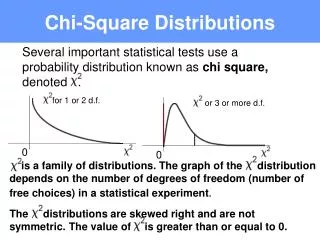
χ-square distribution df = 2 df = 4 df = 10
distribution • Goodness of fit • Test for homogeneity • Test for independence
Goodness of Fit • Testing one categorical value from a single population • Example: • A manufacturer of baseball cards claims • 30% of all cards feature rookies • 60% feature veterans • 10% feature all-stars Reference: http://stattrek.com/Lesson3/ChiSquare.aspx
Assumptions • Data is collected from a simple random sample (SRS) • Population is at least 10 times larger than sample • Variable is categorical • Expected value for each level of the variable is at least 5
Steps in the Process • State the hypothesis • Form an analysis plan • Analyze sample data • Interpret results
Goodness of Fit • State the hypothesis • Null: The data are consistent with a specified distribution • Alternative: The data are not consistent with a specified distribution • At least one of the expected values is not accurate • Baseball card example • 1
Goodness of Fit • Analysis Plan • Specify the significance level • Determine the test method • Goodness of fit • Independence • Homogeneity
Goodness of Fit • Analyze the sample data • Find the degrees of freedom • d.f.= k-1, where k=the number of levels for the distribution • Determine the expected frequency counts • Expected frequency (E) = sample size x hypothesized proportion • Determine the test statistic • Interpret the results
Goodness of fit example Problem • Acme Toy Company prints baseball cards. The company claims that 30% of the cards are rookies, 60% veterans, and 10% are All-Stars. The cards are sold in packages of 100. • Suppose a randomly-selected package of cards has 50 rookies, 45 veterans, and 5 All-Stars. Is this consistent with Acme's claim? Use a 0.05 level of significance.
Using Excel to find • Determine • Create 2 columns: n and p, and enter appropriate values • In the 3rd column:
Another G of F problem • Poisson Distribution • Automobiles leaving the paint department of an assembly plant are subjected to a detailed examination of all exterior painted surfaces. • For the most recent 380 automobiles produced, the number of blemishes per car is summarized below. • Level of significance:
Using Excel to find • Determine • Add a 4th column to the spreadsheet: • In the 5th column, calculate each element of the statistic • =(D2-C2)^2/C2 • Sum the values of the 5th column • This is the value, the test statistic • Use the calculator to find the value of p, and interpret the test results.
Test for homogeneity • Single categorical variable from 2 populations • Test if frequency counts are distributed identically across both populations • Example: Survey of TV viewing audiences. Do viewing preferences of men and women differ significantly? • We make the same assumptions we did for the goodness of fit test • Data is collected from a simple random sample (SRS) • Population is at least 10 times larger than sample • Variable is categorical • Expected value for each level of the variable is at least 5 • We use the same approach to testing
State the hypothesis • Data collected from r populations • Categorical variable has c levels • Null hypothesis is that each population has the same proportion of observations, i.e.: H0: Plevel1, pop 1 = Plevel1, pop 2 =… = Plevel1. pop r H0; Plevel2, pop 1 = Plevel2, pop 2 - … = Plevel2, pop r … H0: Plevelc, pop 1 = Plevelc, pop 2=…=Plevelc, pop r • Alternative hypothesis: at least one of the null statements if false
Analyze the sample data • Find • Degrees of freedom • Expected frequency counts • Test statistic () • p-value or critical value
Analyze the sample data • Degrees of freedom • d.f.=(r-1) x (c-1) • Where • r= number of populations • c= number of categorical values
Analyze the sample data • Expected frequency counts • Computed separately for each population at each categorical variable • Where: • = expected frequency count of each population • = number of observations from each population • = number of observations from each category/treatment level
Analyze the sample data • Determine the test statistic • Determine the p-value or critical value
Test for homogeneity Problem • In a study of the television viewing habits of children, a developmental psychologist selects a random sample of 300 fifth graders - 100 boys and 200 girls. Each child is asked which of the following TV programs they like best.
State the hypotheses • Null hypothesis: The proportion of boys who prefer Family Guy is identical to the proportion of girls. Similarly, for the other programs. Thus: H0: Pboys who like Family Guy = Pgirls who like Family Guy H0: Pboys who like South Park = Pgirls who like South Park H0: Pboys who like The Simpsons = Pgirls who like The Simpsons • Alternative hypothesis: At least one of the null hypothesis statements is false.
Analysis plan • Compute • Degrees of freedom • Expected frequency counts • Chi-square test statistic • Degrees of freedom • Where: • = number of population elements • = number of categories/treatment levels • In this case
Analysis plan Compute the expected frequency counts Er,c = (nr * nc) / nE1,1 = (100 * 100) / 300 = 10000/300 = 33.3E1,2 = (100 * 110) / 300 = 11000/300 = 36.7E1,3 = (100 * 90) / 300 = 9000/300 = 30.0E2,1 = (200 * 100) / 300 = 20000/300 = 66.7E2,2 = (200 * 110) / 300 = 22000/300 = 73.3E2,3 = (200 * 90) / 300 = 18000/300 = 60.0
Analysis plan • Determine the test statistic
Analysis plan • p-value • use the Chi-Square Distribution Calculator to find P(Χ2> 19.91) = 1.0000 • Interpret the results
Test for independence • Almost identical to test for homogeneity • Test for homogeneity: Single categorical variable from 2 populations • Test for independence: 2 categorical variables from a single population • Determine if there is a significant association between the 2 variables • Example • Voters are classified by gender and by party affiliation (D,R,I). • Use X2 test to determine if gender is related to voting preference (are the variables independent?)
Test for independence • Same assumptions • Same approach to testing • Hypotheses • Suppose variable A has r levels and variable B has c levels. The null hypothesis states that knowing the level of A does not help you predict the level of B. The variables are independent. • H0: Variables A and B are independent • Ha: Variables A and B are not independent • Knowing A will help you predict B • Note: Relationship does not have to be causal to show dependence
Test for independence Problem • A public opinion poll surveyed a simple random sample of 1000 voters. Respondents were classified by gender (male or female) and by voting preference (Republican, Democrat, or Independent). Do men’s preferences differ significantly from women’s?
Test for independence • Hypotheses • H0: Gender and voting preferences are independent. • Ha: Gender and voting preferences are not independent. • Analyze sample data • Degrees of freedom • Expected frequency counts • Chi-square statistic • p-value or critical value • Interpret the results