Download
1 / 57
570 likes | 702 Views
Continuous Time and Resource Uncertainty. CSE 574 Lecture Spring ’03 Stefan B. Sigurdsson. (Big Mars Rover Picture). Lecture Overview. Context Classical planning The Mars Rover domain Relaxing the assumptions Q: What’s so different? Innovation Discussion. (Shakey Picture).

E N D
Continuous Time and Resource Uncertainty CSE 574 Lecture Spring ’03 Stefan B. Sigurdsson
Lecture Overview Context • Classical planning • The Mars Rover domain • Relaxing the assumptions • Q: What’s so different? Innovation Discussion
(Shakey Picture) Slide shamelessly lifted from http://www.cs.nott.ac.uk/~bsl/G53DIA/Slides/Deliberative-architectures-I.pdf
STRIPS-Like Planning Actions World Description Conjunctive precondition STRIPS operators Conj. effect (add/delete) Instantaneous Sequential Deterministic Propositional logic Closed world assumption Finite and static Complete knowledge Discrete time No exogenous effects Goal Description Attainment – “Win or lose” Conjunctions of positive literals Plan…
The Mars Rover Domain Robot control, with… • Positioning and navigation • Complex choices (goals and actions) • Rich utility model • Continuous time and concurrency • Uncertain resource consumption • Metric quantities • Very high stakes! But alone in a finite, static universe
Resources? Metric Quantities? What are those? Various flavors: • Exclusive (camera arm) • Shared (OS scheduling) • Metric quantity (fuel, power, disk space) Uncertainty
Is This Really A Planning Problem? Better suited to OR/DT-type scheduling? • Time, resources, metric quantities, concurrency, complicated goals/rewards… Complex, inter-dependent activities • Select, calibrate, use, reuse, recalibrate sensors • OR-type scheduling can’t handle rich choices Insight: Maybe we can borrow some tricks?
Can Planners Scale Up? Large plans • Sequences of ~ 100 actions Where do we start? • POP? • MDP? • Graph/SATplan?
Can Planners Scale Up? Large plans • Sequences of ~ 100 actions Where do we start? • POP? (Branch factors are too big) • MDP? • Graph/SATplan?
Can Planners Scale Up? Large plans • Sequences of ~ 100 actions Where do we start? • POP? (Branch factors are too big) • MDP? (Complete policy is too large) • Graph/SATplan?
Can Planners Scale Up? Large plans • Sequences of ~ 100 actions Where do we start? • POP? (Branch factors are too big) • MDP? (Complete policy is too large) • Graph/SATplan? (Discrete representations)
Which Extensions First? Metric quantities • Time • Resources Resource Uncertainty Concurrency What about non-determinism? Reasonable for Graphplan?
A (Very Incomplete)Research Timeline 1971 STRIPS (Fikes/Nilson) 1989 ADL (Pednault) 1991 PEDESTAL (McDermott) 1992 UCPOP (Penberthy/Weld) 1992 SENSp (Etzioni et al.) CNLP (Peot/Smith) 1993 Buridan (Kushmerick et al.) 1994 C-Buridan (Draper et al.) JIC Scheduling (Drummond et al.) HSTS (Muscettola) Zeno (Penb./Weld) Softbots (Weld/Etzioni) MDP (Williamson/Hanks) 1995 DRIPS (Haddawy et al.) IxTeT (Laborie/Ghallab) 1997 IPP (Koehler et al.) 1998 PGraphplan (Blum/Langford) Weaver (Blythe) PUCCINI (Golden) CGP (Smith/Weld) SGP (Weld et al.) Pgraphplan (Blum/Langford) 1999 Mahinur (Onder/Pollack) ILP-PLAN (Kautz/Walzer) TGP (Smith/Weld) LPSAT (Wolfman/Weld) 2000 T-MDP (Boyan/Littman) HSTS/RA (Jónsson et al.) Since then? Not implemented ADL impl. Sensing Conformant Contingent Planning + scheduling Metric time/resources Safe planning Dec. theory goals Uncertain utility Shared resources Uncertain/dynamic Sensing Conformant Contingent Resources Resources
STRIPS UCPOP CGP CNLP SENSp Buridan Weaver C-Buridan MDP PO-MDP S-MDP T-MDP F-MDP LPSAT Mars Rover Domain Assumptions Classical Expressive logic Non-determinism Observation Goal model Plan utility Durative actions Complex concurrence Continuous time Metric quantities Branching factor Resource uncertainty Resource constraints Goal selection Safe planning Exogenous events Select contingencies Serialized goals? Bleeding edge
Brain-teaser: Domain Spec State space S • Cartesian product of continuous and discrete axes (time, position, achievements, energy…) Initial state si • Probability distribution Domain theory • Concurrent, non-deterministic, uncertain What else? (S, si, , …)
Brain-teaser: Kalman Filters Curiously missing from the paper we read (?) 1983 Kalman filters paper: Voyager enters Jupiter orbit through a 30 second window after 11 years in space Hugh Durrant-Whyte’s robots Why not for the Mars Rover?
Context Summary Complex, exciting domain Pushes the planning envelope • Expression • Scaling Where do we start?
Lecture Overview Context Innovation • Just-in-case planning • Incremental contingency planning Discussion
Just-In-Case Planning Motivated by domain characteristics • Metric quantities • Large branch factors Implications • Not plan, not policy • Expanded plan What about concurrency?
Branch Heuristics Most probable failure point (scheduling) Highest utility branch point (planning) What is the intrinsic difference?
Incremental Contingency Planning Algorithm Input: Domain description and master plan Output: Highest-utility branch point Algorithm: • Compute value, estimate resources during master plan • Approximate branch point utilities • Select highest-utility branch point • Solve w/ new initial, goal conditions • Repeat while necessary
Branch Utility Approximation … without constructing plan • Construct a plan graph • Back-propagate utility functions through plan graph, instead of regression searching • Compute branch point utilities throughout input plan
Back-Propagating Distributions Mausam: “Some parts of the paper are tersely written, which make it a little harder to understand. I got quite confused in the discussion of utility propagation. It would have been nicer had they given some theorems about the soundness of their method.” Well, me too
Back-Propagating Distributions (10, 15) A B q g (10, 15) p C r (3, 3) E g’ (2, 2) D s t (1, 5)
1 Back-Propagating Distributions 5 (10, 15) A B q g (10, 15) p C r (3, 3) E g’ (2, 2) D s t (1, 5)
1 Back-Propagating Distributions 5 15 5 (10, 15) A B q g (10, 15) p C r (3, 3) E g’ (2, 2) D s t (1, 5)
1 Back-Propagating Distributions 5 5 15 5 25 (10, 15) A B q g (10, 15) p C r (3, 3) E g’ (2, 2) D s t (1, 5)
1 1 Back-Propagating Distributions 5 5 15 5 25 (10, 15) A B q g (10, 15) p C r (3, 3) E g’ (2, 2) D s t (1, 5) 2
1 1 1 1 Back-Propagating Distributions 5 5 15 5 25 (10, 15) A B q g (10, 15) t p C 2 r (3, 3) E g’ (2, 2) D s t (1, 5) r 2 2
1 1 1 1 Back-Propagating Distributions 5 5 15 5 25 (10, 15) A B q g (10, 15) t p C 2 r (3, 3) E g’ (2, 2) D s t (1, 5) r r 2 1 5 2
1 1 1 1 Back-Propagating Distributions 5 5 15 5 25 (10, 15) A B q g (10, 15) t p C 2 t r 1 (3, 3) E 5 g’ (2, 2) D s t (1, 5) r r 2 1 5 2
1 1 1 1 Back-Propagating Distributions t 6 5 5 1 + 15 5 15 25 25 15 (10, 15) A B q g (10, 15) t p C 2 t r 1 (3, 3) E 5 g’ (2, 2) D s t (1, 5) r r 2 1 5 2
1 1 1 1 Back-Propagating Distributions t 6 5 5 1 + 15 5 15 25 25 15 (10, 15) 6 t 5 1 + A B 5 25 25 15 q g (10, 15) t p C 2 t r 1 (3, 3) E 5 g’ (2, 2) D s t (1, 5) r r 2 1 5 2
1 1 1 Back-Propagating Distributions t 6 5 5 1 + 15 5 15 25 25 15 (10, 15) 6 t 5 1 + A B g 5 25 25 15 q (10, 15) t r p 1 1 + C 2 5 t r 1 (3, 3) E 5 g’ (2, 2) D s t (1, 5) r r 2 1 5 2
1 1 1 Back-Propagating Distributions t 6 5 5 1 + 15 5 15 25 25 15 (10, 15) 6 t 5 1 + A B g 5 25 25 15 q (10, 15) t p 1 1 + C 2 5 t r 1 (3, 3) E 5 g’ (2, 2) D s t (1, 5) r r 2 1 5 2
1 1 1 Back-Propagating Distributions t 6 5 5 1 + 15 5 15 25 25 15 (10, 15) 6 t 5 1 + A B g 5 25 25 15 q (10, 15) t p 1 1 + C t 2 5 r 1 1 + (3, 3) E 5 8 g’ (2, 2) D s t (1, 5) r r 2 1 5 2
1 1 1 Back-Propagating Distributions t 6 5 5 1 + 15 5 15 15 25 25 25 15 (10, 15) 6 t 5 1 + A B g 5 25 25 15 q (10, 15) t p 1 1 + C t 2 5 r 1 1 + (3, 3) E 5 8 g’ (2, 2) D s t (1, 5) r r 2 1 5 2
1 1 1 Back-Propagating Distributions t 6 5 5 1 + 15 5 15 15 25 25 25 15 (10, 15) 6 t 5 1 + A B g 8 5 25 25 15 q (10, 15) t p 1 1 + C t 2 5 r 1 1 + (3, 3) E 5 8 g’ (2, 2) D s t (1, 5) r r 2 1 5 2
1 1 1 Back-Propagating Distributions t 6 5 5 1 + 15 5 15 15 25 25 25 15 (10, 15) 6 t 5 1 + A B g 8 5 25 25 15 q (10, 15) t p 1 1 + C t 2 5 r 1 1 + (3, 3) E 5 8 g’ (2, 2) D s t (1, 5) r r 1 2 1 8 5 2
1 1 1 Back-Propagating Distributions t 6 5 5 1 + 15 5 15 15 25 25 25 15 (10, 15) 6 t 5 1 + A B g 8 5 25 25 15 q (10, 15) t p 1 1 + C t 2 5 r 1 1 + (3, 3) E 5 8 g’ (2, 2) D s t (1, 5) r r 1 2 1 8 5 2 (CDE)
1 1 1 Back-Propagating Distributions t 6 5 5 1 + 15 5 15 15 25 25 25 15 (10, 15) 6 t 5 1 + A B g 8 5 25 25 15 q (10, 15) t p 1 1 + C t 2 5 r 1 1 + (3, 3) E 5 8 g’ (2, 2) D s t (1, 5) r r 1 2 1 8 5 2 (CDE)
1 1 1 Back-Propagating Distributions t 6 5 5 1 + 15 5 15 15 25 25 25 15 (10, 15) [(DCE) (AB) (DABE)] A B g q (10, 15) t p 1 1 + C t 2 5 r 1 1 + (3, 3) E 5 8 g’ (2, 2) D s t (1, 5) [(CDE) (ABDE)] r r 2 1 5 2
1 1 1 Back-Propagating Distributions t 6 5 5 1 + 15 5 15 15 25 25 25 15 (10, 15) 6 A B 5 1 g q 6 25 26 (10, 15) t (DCE, AB, DABE) p 1 1 + C t 2 5 r 1 1 + (3, 3) E 5 8 g’ (2, 2) D s t (1, 5) 6 r r 1 2 1 8 25 5 2 (CDE, ABDE)
Utility Estimation 6 5 1 6 25 26 (DCE, AB, DABE) p s 6 1 8 25 (CDE, ABDE)
Utility Estimation 6 5 1 MAX operator: 6 25 26 (DCE, AB, DABE) p 6 1 6 25 s (DCE, ABDE) 6 1 8 25 (CDE, ABDE)
Utility Estimation 6 5 1 MAX operator: 6 25 26 (DCE, AB, DABE) p 6 1 6 25 s (DCE, ABDE) 6 1 8 25 (CDE, ABDE) (Then combine w/Monte Carlo results)