Download
1 / 8
80 likes | 109 Views
Continuous-Time Convolution. Impulse Response. Impulse response of a system is response of the system to an input that is a unit impulse (i.e., a Dirac delta functional in continuous time) When initial conditions are zero, this differential equation is LTI and system has impulse response.

E N D
Impulse Response • Impulse response of a system is response of the system to an input that is a unit impulse (i.e., a Dirac delta functional in continuous time) • When initial conditions are zero, this differential equation is LTI and system has impulse response
x(t) t t=nDt Dt System Response • Signals as sum of impulses • But we know how to calculate the impulse response ( h(t) ) of a system expressed as a differential equation • Therefore, we know how to calculate the system output for any input, x(t)
Graphical Convolution Methods • From the convolution integral, convolution is equivalent to • Rotating one of the functions about the y axis • Shifting it by t • Multiplying this flipped, shifted function with the other function • Calculating the area under this product • Assigning this value to f1(t) * f2(t) at t
f(t) g(t) 3 2 * t t 2 -2 2 3 g(t-t) 2 f(t) t 2 -2 + t 2 + t Graphical Convolution Example • Convolve the following two functions: • Replace t with t in f(t) and g(t) • Choose to flip and slide g(t) since it is simpler and symmetric • Functions overlap like this: t
3 g(t-t) 2 f(t) t 2 -2 + t 2 + t 3 g(t-t) 2 f(t) t 2 -2 + t 2 + t Graphical Convolution Example • Convolution can be divided into 5 parts • t < -2 • Two functions do not overlap • Area under the product of thefunctions is zero • -2 t < 0 • Part of g(t) overlaps part of f(t) • Area under the product of thefunctions is
3 g(t-t) 2 f(t) t 2 -2 + t 2 + t 3 g(t-t) 2 f(t) t 2 -2 + t 2 + t Graphical Convolution Example • 0 t < 2 • Here, g(t) completely overlaps f(t) • Area under the product is just • 2 t < 4 • Part of g(t) and f(t) overlap • Calculated similarly to -2 t < 0 • t 4 • g(t) and f(t) do not overlap • Area under their product is zero
Graphical Convolution Example • Result of convolution (5 intervals of interest): No Overlap Partial Overlap Complete Overlap Partial Overlap No Overlap y(t) 6 t -2 0 2 4